Structured Prediction part two - Implementing a linear-chain CRF
In this part of the series of posts on structured prediction with conditional random fields (CRFs) we are going to implement all the ingredients that were discussed in part 1. Recall that we discussed how to model the dependencies among labels in sequence prediction tasks with a linear-chain CRF. Now, we will put a CRF on top of a neural network feature extractor and use it for part-of-speech (POS) tagging.
Everything below is inspired by this paper by Ma & Hovy (although we’ll train on a smaller dataset for time’s sake and we’ll skip much of the components since it’s not about performance but more about educational value), and the implementation has lots of parts that come from the AllenNLP implementation, so if it’s simply a good implementation you’re looking for, take a look at that one. If you’d like to understand how it works from scratch, keep on reading. Bear with me here, I discuss everything rather in detail and try not to skip over anything, from batching and broadcasting to changing the forward-recursion of BP for a cleaner implementation, so if you rather want a succint blogpost you might want to choose one of the great other options that are also out there! Alternatively, there are some sections you can skip if they’re clear, like batching and broadcasting. Let’s start!
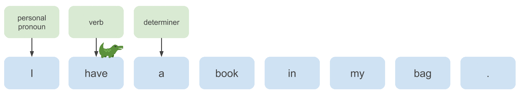
To learn a model that can annotate examples like the one above with predicted POS tags, we need to extract useful features from the input sequence, which we will do with a bidirectional LSTM (motivated below). Then what we’ll implement in this post is:
-
An
Encodermodel that holds our feature extractor (the bidirectional LSTM). -
A
ChainCRFmodel that implements all the CRF methods, like belief propagation (BP) and Viterbi decoding.
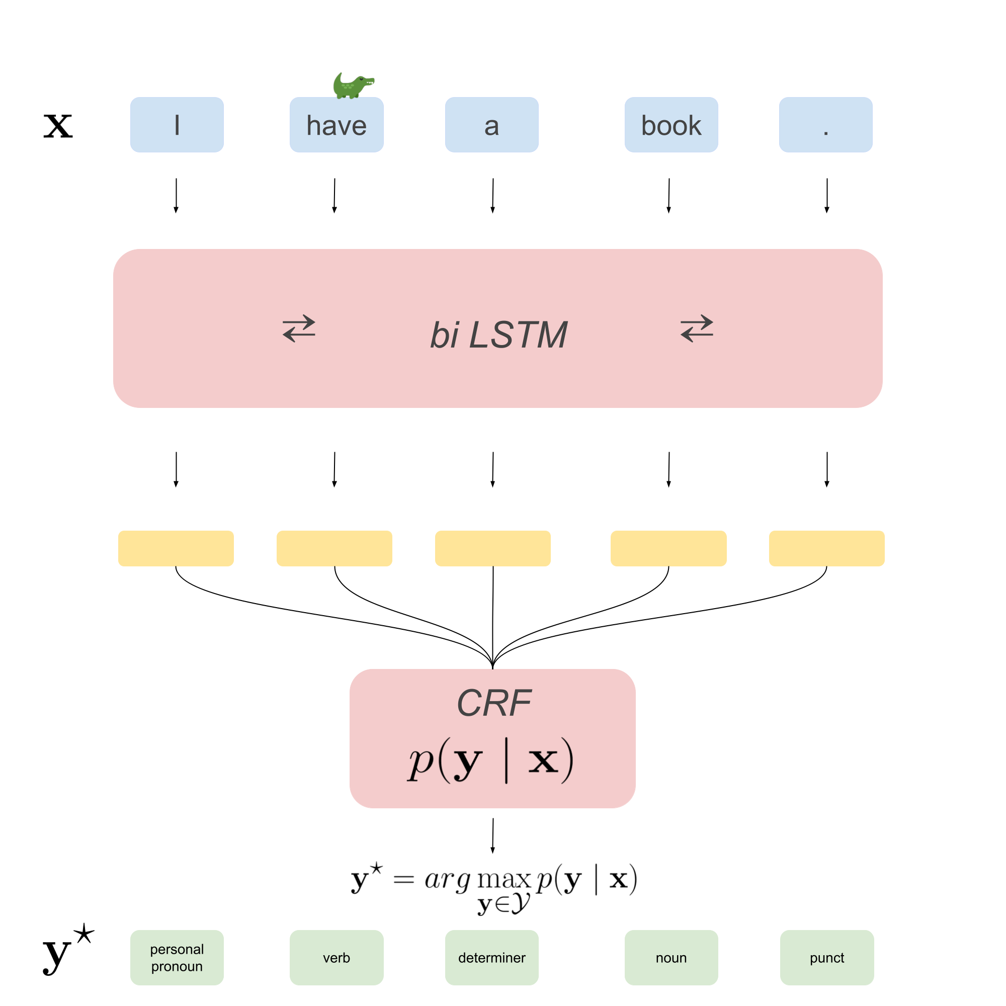
The end-to-end model we get by walking through this post is depicted in the image below.
To train this model end-to-end we will use the negative log-likelihood (NLL) loss function, which is simply the negated log-likelihood that was given in part 1 of this series. Given some example input-output pairs \((\mathbf{x}^{(i)}, \mathbf{y}^{(i)})_{i=1}^N\), the NLL of the entire dataset is:
\[\begin{aligned} \text{NLL} = -\log \mathcal{L}(\boldsymbol{\theta}) &= - \sum_{i=1}^{N} \log p(\mathbf{y}^{(i)} \mid \mathbf{x}^{(i)}) \\ &= \sum_{i=1}^{N}\log\left(Z(\mathbf{x}^{(i)})\right) - \sum_{i=1}^{N}\left(\sum_{t=1}^m \boldsymbol{\theta}_1 f(y_t^{(i)}, \mathbf{x}^{(i)}, t) + \sum_{t=1}^{m-1} \boldsymbol{\theta}_2 f(y_t^{(i)}, y_{t+1}^{(i)})\right) \\ \end{aligned}\]Instead of maximizing the log-likelihood of our data, we will minimize the negative log-likelihood, which is equivalent.
We can use stochastic gradient descent (SGD) with automatic differentiation in PyTorch, meaning we only need the forward-part of the BP algorithm.
Recall that the forward recursion allows calculation of the partition function (\(Z(\mathbf{x})\)), which we need for the NLL. The backward recursion allows calculating the
marginals (which are needed for the gradients). PyTorch takes care of the latter calculation for us (<3 PyTorch). Also, since
we’ll be using SGD on minibatches the above sum will go over \(B < N\) examples randomly sampled from the dataset, for batch size \(B\).
Let’s start with feature extraction and defining \(\boldsymbol{\theta}_1\), \(\boldsymbol{\theta}_2\), \(f(y_t, \mathbf{x}, t)\), and \(f(y_t, y_{t+1})\).
Preliminaries
If you want to run the code used in this post yourself, make sure to install PyTorch >= 1.7.0, Python 3.6, and TorchNLP >= 0.5.0.
Feature Extraction
There are some desiderata for our features. The function \(f(y_t, \mathbf{x}, t)\) signifies that we want each tag in the output sequence \(y_t\) to be informed about (i.e., depend on) the entire input sequence \(\mathbf{x}\), but also on the current word at time \(t\). Furthermore, \(f(y_t, y_{t+1})\) tells us that we want each next output tag \(y_{t+1}\) to depend on the previous tag \(y_{t}\). Parametrizing the former part, we take \(\boldsymbol{\theta}_1f(y_t, \mathbf{x}, t)\) to be the output of a bidirectional LSTM projected down to the right dimension with a linear layer:
\[\begin{aligned} \mathbf{\bar{H}} &= \text{biLSTM}(\mathbf{x}) \\ \mathbf{H} &= \mathbf{\bar{H}}\mathbf{W} + \mathbf{b} \end{aligned}\]In the above, \(\mathbf{x} \in \mathbb{R}^{m}\) is our input sequence, \(\mathbf{\bar{H}} \in \mathbb{R}^{m \times 2d_h}\) the hidden vectors for each input word \(x_t\) stacked into a matrix, with \(d_h\) the hidden dimension of the LSTM (doubled because a bidirectional LSTM is essentially two LSTMs processing the input sequence from left-to-right and right-to-left). \(\mathbf{W} \in \mathbb{R}^{2d_h \times |S|}\) a matrix of parameters that projects the output to the right dimension, namely \(|S|\) values for each input word \(x_t\). The t-th row of \(\mathbf{H} \in \mathbb{R}^{m \times |S|}\) (let’s define that by \(\mathbf{H}_{t*}\)) then holds the features for the t-th word (\(x_t\)) in the input sequence. These values reflect \(\boldsymbol{\theta}_1f(y_t, \mathbf{x}_t, t)\) for each possible \(y_t\), since they depend on the entire input sequence \(\mathbf{x}\), but are specific to the current word at time \(t\).
\[\boldsymbol{\theta}_1f(y_t, \mathbf{x}_t, t) = \mathbf{H}_{t,y_t}\]Using PyTorch, we can code this up in a few lines. As is common in computational models of language, we will assign each
input token a particular index and use dense word embeddings that represent each word in our input vocabulary. We reserve
index 0 for the special token <PAD>, which we need later when we will batch our examples, grouping together examples
of different length \(m\).
Strictly speaking btw, our bi-LSTM does not take \(\mathbf{x}\) as input but \(\mathbf{E}_{x_t*}\), where \(\mathbf{E}\) is the matrix of embedding parameters of size \(|I| \times d_e\) (where \(I\) is the input vocabulary size, or the number of unique input words). So if \(x_t = 3\) (index 3 in our vocabulary, which might be mapping to book for example), \(\mathbf{E}_{x_t*}\) takes out the corresponding embedding of size \(d_e\).
class Encoder(nn.Module):
  """
  A simple encoder model to encode sentences. Bi-LSTM over word embeddings.
  """
  def __init__(self, vocabulary_size: int, embedding_dim: int,
                     hidden_dimension: int, padding_idx: int):
    super(Encoder, self).__init__()
    # The word embeddings.
    self.embedding = nn.Embedding(num_embeddings=vocabulary_size,
                                  embedding_dim=embedding_dim,
                                  padding_idx=padding_idx)

    # The bi-LSTM.
    self.bi_lstm = nn.LSTM(input_size=embedding_dim,
                           hidden_size=hidden_dimension, num_layers=1,
                           bias=True, bidirectional=True)

  def forward(self, sentence: torch.Tensor) -> torch.Tensor:
    """
    :param sentence: input sequence of size [batch_size, sequence_length]
    Returns: tensor of size [batch_size, sequence_length, hidden_size * 2]
    the hidden states of the biLSTM for each time step.
    """
    embedded = self.embedding(sentence)
    # embedded: [batch_size, sequence_length, embedding_dimension]

    output, (hidden, cell) = self.bi_lstm(embedded)
    # output: [batch_size, sequence_length, hidden_size * 2]
    # hidden: [batch_size, hidden_size * 2]
    # cell: [batch_size, hidden_size * 2]
    return output
That’s all we need to do to extract features from out input sequences! Later in this post we will define \(\boldsymbol{\theta}_2\)
and \(f(y_t, y_{t+1})\), which are part of the actual CRF. First, we’ll set up our Tagger-module which takes the encoder,
the CRF (to implement later), and outputs the negative log-likelihood and a predicted tag sequence.
The Tagger
Below we can find the Tagger module. This is basically the class that implements the model as depicted in the image
above. The most interesting part is still missing (namely the ChainCRF-module, but also the Vocabulary-module), but we’ll get to those. The
forward pass of the Tagger takes an input sequence, a target sequence, and an input mask (we’ll get to what that is
when we discuss batching), puts the input sequence through the encoder and the CRF, and outputs the NLL loss, the score (
which is basically the nominator of \(p(\mathbf{y} \mid \mathbf{x})\)), and the tag_sequence obtained by decoding with viterbi.
If you don’t have a feeling of what the parameters input_mask and input_lengths in the module should be, don’t worry,
that will be discussed in the section ‘sequence batching’ below.
class Tagger(nn.Module):
  """
  A bi-LSTM-CRF POS tagger.
  """

  def __init__(self, input_vocabulary: Vocabulary,
               target_vocabulary: Vocabulary,
               embedding_dimension: int, hidden_dimension: int):
    super(Tagger, self).__init__()
    # The Encoder to extract features from the input sequence.
    self.encoder = Encoder(vocabulary_size=input_vocabulary.size,
                           embedding_dim=embedding_dimension,
                           hidden_dimension=hidden_dimension,
                           padding_idx=input_vocabulary.pad_idx)

    # The linear projection (with parameters W and b).
    self.encoder_to_tags = nn.Linear(hidden_dimension * 2,
                                     target_vocabulary.size)

    # The linear-chain CRF.
    self.tagger = ChainCRF(num_tags=target_vocabulary.size,
                           tag_vocabulary=target_vocabulary)

  def forward(self, input_sequence: torch.Tensor,
              target_sequence: torch.Tensor,
              input_mask: torch.Tensor, input_lengths: torch.Tensor):
    """
    :param input_sequence: input sequence of size
            [batch_size, sequence_length, input_vocabulary_size]
    :param target_sequence: POS tags target, [batch_size, sequence_length]
    :param input_mask: padding-mask, [batch_size, sequence_length]
    :param input_lengths: lengths of each example in the batch [batch_size]
    Returns: A tuple containing the loss per example, the score per example
    and a predicted taq sequence per example in the batch.
    """
    # input_sequence: [batch_size, sequence_length, input_vocabulary_size]
    lstm_features = self.encoder(input_sequence)
    # lstm_features: [batch_size, sequence_length, hidden_dimension*2]

    crf_features = self.encoder_to_tags(lstm_features)
    # crf_features: [batch_size, sequence_length, target_vocabulary_size]

    loss, score, tag_sequence = self.tagger(input_features=crf_features,
                                            target_tags=target_sequence,
                                            input_mask=input_mask,
                                            input_lengths=input_lengths)
    # loss, score: scalars
    # tag_sequence: [batch_size, sequence_length]
    return loss, score, tag_sequence
OK, now we can finally get to the definition of \(\boldsymbol{\theta}_2\) and \(f(y_t, y_{t+1})\), and the implementation of the linear-chain CRF!
Implementing a Linear-Chain CRF
We want \(f(y_t, y_{t+1})\) to represent the likelihood of some tag \(y_{t+1}\) following \(y_t\) in the sequence, which
can be interpreted as transition likelihood from one tag to another. We assumed the parameters \(\boldsymbol{\theta}_2\) are shared
over time (meaning they are the same for each \(t \in \{1, \dots, m-1\}\)), and thus we can simply define a matrix of transition ‘probabilities’ from each tag to another tag.
We define \(\boldsymbol{\theta}_2f(y_t, y_{t+1}) = \mathbf{T}_{y_t,y_{t+1}}\), meaning the \(y_t\)-th row (recall that \(y_t\) is an index that represents a tag) and \(y_{t+1}\)-th column of a matrix \(\mathbf{T}\).
This matrix \(\mathbf{T}\) will be of size \((|S| + 2) \times (|S| + 2)\). The 2 extra tags are the <ROOT> and the <EOS> tag.
We need some tag to start of the sequence and to end the sequence, because we want to take into account the probability of a particular tag being the
first tag of a sequence, and the probability of a tag being the last tag. For the former we will use <ROOT>, and a for the latter we’ll use <EOS>.
In this part we will implement:
-
The forward-pass of belief propagation (
ChainCRF.forward_belief_propagation(...)), calculating the partition function (i.e., the denominator of \(p(\mathbf{y} \mid \mathbf{x})\)). -
Calculating the log-nominator of \(p(\mathbf{y} \mid \mathbf{x})\) (
ChainCRF.score_sentence(...)) -
Decoding to get the target sequence prediction (
ChainCRF.viterbi_decode(...))
Below, you’ll find the ChainCRF class that holds all these methods. The matrix of transition probabilities \(\mathbf{T}\)
is initialized below as log_transitions (note that \(\mathbf{T}\) are actually the log-transition probabilities because in the CRF equations they are \(\exp(\boldsymbol{\theta}_2f(y_t, y_{t+1})) = \exp\mathbf{T}_{y_t,y_{t+1}}\)), and we hard-code the transition probabilities from any \(y_t\) to the <ROOT>
tag to be -10000 because this should not be possible (and this becomes 0 in the CRF equation: exp(log_transitions) gives \(\exp-10000 \approx 0\)).
We do the same for any transition from <EOS> to any other tag. The class below implements the methods to calculate the NLL loss, and the total forward-pass of the CRF that returns this loss as well as a predicted tag sequence. In the sections below we will implement the necessary methods for our linear-chain CRF, starting with belief propagation.
 class ChainCRF(nn.Module):
      """
      A linear-chain conditional random field.
      """

      def __init__(self, num_tags: int, tag_vocabulary: Vocabulary):
        super(ChainCRF, self).__init__()

        self.tag_vocabulary = tag_vocabulary
        self.num_tags = num_tags + 2 # +2 for <ROOT> and <EOS>
        self.root_idx = tag_vocabulary.size
        self.end_idx = tag_vocabulary.size + 1

        # Matrix of transition parameters.  Entry (i, j) is the score of
        # transitioning *from* i *to* j.
        self.log_transitions = nn.Parameter(torch.randn(self.num_tags,
                                                        self.num_tags))

        # Initialize the log transitions with xavier uniform (TODO: refer)
        self.xavier_uniform()

        # These two statements enforce the constraint that we never transfer
        # to the start tag and we never transfer from the stop tag
        self.log_transitions.data[:, self.root_idx] = -10000.
        self.log_transitions.data[self.end_idx, :] = -10000.

      def xavier_uniform(self, gain=1.):
        torch.nn.init.xavier_uniform_(self.log_transitions)

      def forward_belief_propagation(self, input_features: torch.Tensor,
                                    input_mask: torch.Tensor) -> torch.Tensor:
        raise NotImplementedError()

      def score_sentence(self, input_features: torch.Tensor,
                        target_tags: torch.Tensor,
                        input_mask: torch.Tensor) -> torch.Tensor:
        raise NotImplementedError()

      def viterbi_decode(self, input_features: torch.Tensor,
                               input_lengths: torch.Tensor) -> Tuple[
                                                        torch.Tensor,
                                                        torch.Tensor]:
        raise NotImplementedError()

      def negative_log_likelihood(self, input_features: torch.Tensor,
                                  target_tags: torch.Tensor,
                                  input_mask: torch.Tensor) -> torch.Tensor:
        """
        Returns the NLL loss.
        :param input_features: the features for each input sequence
                [batch_size, sequence_length, feature_dimension]
        :param target_tags: the target tags
                [batch_size, sequence_length]
        :param input_mask: the binary mask determining which of
                the input entries are padding [batch_size, sequence_length]
        """
        partition_function = self.forward_belief_propagation(
                                    input_features=input_features,
                                    input_mask=input_mask)
        log_nominator = self.score_sentence(
                                    input_features=input_features,
                                    target_tags=target_tags,
                                    input_mask=input_mask)
        return partition_function - log_nominator

      def forward(self, input_features: torch.Tensor,
                  target_tags: torch.Tensor,
                  input_mask: torch.Tensor,
                  input_lengths: torch.Tensor) -> Tuple[torch.Tensor,
                                                        torch.Tensor,
                                                        torch.Tensor]:
        """
        The forward-pass of the CRF, which calculates the NLL loss and
        returns a predicted sequence.
        :param input_features: features for each input sequence
                [batch_size, sequence_length, feature_dimension]
        :param target_tags: the target tags
                [batch_size, sequence_length]
        :param input_mask: the binary mask determining which of
                the input entries are padding [batch_size, sequence_length]
        :param input_lengths: the sequence length of each example in the
                batch of size [batch_size]
        """
        loss = self.negative_log_likelihood(input_features=input_features,
                                            target_tags=target_tags,
                                            input_mask=input_mask)
        with torch.no_grad():
          score, tag_sequence = self.viterbi_decode(input_features,
                                                    input_lengths=input_lengths)
        return loss, score, tag_sequence
But first, since we implement all these method in batched versions, let’s briefly go over batching.
Sequence Batching
Processing data points in batches has multiple benefits: averaging the gradient over a minibatch in SGD allows playing with the noise you want while training your model (batch size of 1 gives a maximally noisy gradient, batch size of \(N\) is minimally noisy gradient, namely gradient descent without the stochasticity), but also: batching examples speeds up training. This motivates us to implement all the methods for the CRF in batched versions, allowing parallel processing. We can’t parallelize the time-dimension in CRFs unfortunately.
A batch of size 2 would look like this:
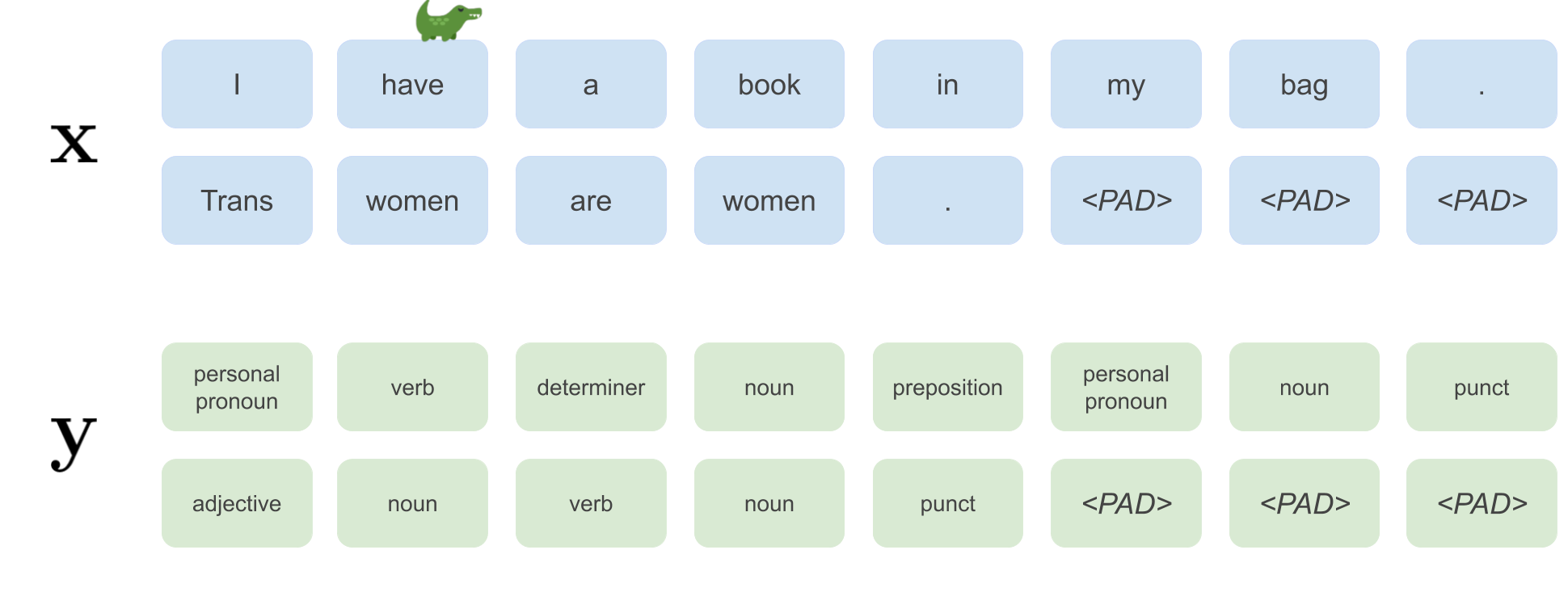
For each batch we will additionally keep track of the lengths in the batch. For the image above a list of lengths would be input_lengths = [8, 5].
For example, batched inputs to our encoder will be of size [batch_size, sequence_length] and outputs of size [batch_size, sequence_length, hidden_dim*2].
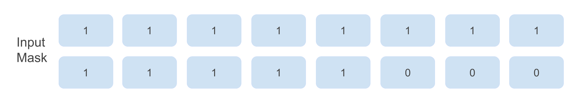
The input mask for the above batch looks like this:
Implementation in log-space, stable ‘‘logsumexp-ing’’ & broadcasting
Before we can finally get into the interesting implementations, we need to talk about two things. Firstly, for calculating the partition function we are going to need to sum a bunch of \(exp(\cdot)\)’s, which might explode. To do this numerically stable, we will use the logsumexp-trick. The log here comes from the fact that we will implement everything in log-space. Numerical stability doesn’t fare well with recursive multiplication of small values (i.e., values between 0 and 1) or large values. In log-space, multiplications become summations, which have less of a risk of becoming too small or too large. Recall that the initialization and recursion in the forward-pass of belief propagation are given by the following equations:
\[\begin{aligned} \alpha(1, y^{\prime}_2) &= \sum_{y^{\prime}_1}\psi(y^{\prime}_1, \mathbf{x}, 1) \cdot \psi(y^{\prime}_1, y^{\prime}_{2}) \\ \alpha(t, y^{\prime}_{t+1}) &\leftarrow \sum_{y^{\prime}_{t}}\psi(y^{\prime}_t, \mathbf{x}, t) \cdot \psi(y^{\prime}_t, y^{\prime}_{t+1})\cdot \alpha(t-1, y^{\prime}_t) \end{aligned}\]First we convert the alpha initialization to log-space:
\[\begin{aligned} \alpha(1, y^{\prime}_2) &= \sum_{y^{\prime}_1}\psi(y^{\prime}_1, \mathbf{x}, 1) \cdot \psi(y^{\prime}_1, y^{\prime}_{2}) \\ \log \alpha(1, y^{\prime}_2) &= \log \sum_{y^{\prime}_1}\psi(y^{\prime}_1, \mathbf{x}, 1) \cdot \psi(y^{\prime}_1, y^{\prime}_{2}) \\ \end{aligned}\]Then we convert the recursion equation to log-space, we plug in the CRF factors, and we see why we get a logsumexp:
\[\begin{aligned} \log \alpha(t, y^{\prime}_{t+1}) &\leftarrow \log \sum_{y^{\prime}_{t}}\psi(y^{\prime}_t, \mathbf{x}, t) \cdot \psi(y^{\prime}_t, y^{\prime}_{t+1})\cdot \exp\log\alpha(t-1, y^{\prime}_t) \\ \log \alpha(t, y^{\prime}_{t+1}) &\leftarrow \log \sum_{y^{\prime}_{t}}\exp\left(\boldsymbol{\theta}_1f(y^{\prime}_t, \mathbf{x}, t) + \boldsymbol{\theta}_2f(y^{\prime}_t, y^{\prime}_{t+1})\right) \cdot \exp\log\alpha(t-1, y^{\prime}_t) \\ \log \alpha(t, y^{\prime}_{t+1}) &\leftarrow \underbrace{\log \sum_{y^{\prime}_{t}}\exp}_{\text{logsumexp}}\left(\boldsymbol{\theta}_1f(y^{\prime}_t, \mathbf{x}, t) + \boldsymbol{\theta}_2f(y^{\prime}_t, y^{\prime}_{t+1}) + \log\alpha(t-1, y^{\prime}_t)\right) \end{aligned}\]Now what logsumexp does is rewrite this as follows. Let everything inside the \(exp(\cdot)\) above for simplicity be \(q_t\):
\[\begin{aligned} \log \sum_{y^{\prime}_{t}}\exp(q_t) &= \log \sum_{y^{\prime}_{t}}\exp(q_t - c + c) \\ &= \log \sum_{y^{\prime}_{t}}\exp(q_t - c)\exp(c) \\ &= \log \exp(c)\sum_{y^{\prime}_{t}}\exp(q_t - c) \\ &= c + \log\sum_{y^{\prime}_{t}}\exp(q_t - c) \\ \end{aligned}\]If we take the constant \(c\) to be the maximum value that \(q_t\) can take in the sum, the summation becomes stable. See below the code that implements this, adapted from AllenNLP.
def logsumexp(tensor: torch.Tensor, dim: int=-1) -> torch.Tensor:
    """
    A numerically stable computation of logsumexp. This is mathematically
    equivalent to `tensor.exp().sum(dim).log()`.
    This function is typically used for summing log probabilities.
    :param tensor: A tensor of arbitrary size.
    :param dim: The dimension of the tensor to apply the logsumexp to.
    """
    max_score, _ = tensor.max(dim)
    stable_vec = tensor - max_score.unsqueeze(dim)
    return max_score + (stable_vec.exp().sum(dim)).log()
Secondly, we need to talk about broadcasting. Broadcasting over dimensions is conceptually the same thing as matrix multiplication,
but then by summing. For example, if we sum a + b = c where \(a \in \mathbb{R}^{2 \times 1}\) and \(b \in \mathbb{R}^{1 \times 2}\)
the result will be \(c \in \mathbb{R}^{2 \times 2}\):
You can use broadcasting if you have a value that you want to add to every index of a vector, like in the above case 1 is added to 3 and 4 for the top row and 2 to 3 and 4 for the bottom row.
Forward Belief Propagation
In this section we will implement the forward-pass of belief propagation, which we need to calculate part of the NLL loss (namely \(\log\left(Z(\mathbf{x}^{(i)})\right)\)).
We are implementing the forward recursion in a batched version, meaning that the loop over time goes from \(t=1\) to \(m-1\) for the largest \(m\) in the batch. Some sequences might already end somewhere earlier in the loop, which is why we will mask out the recursion for those sequences and retain the old \(\alpha\) variables for them. Implementing batched forward belief propagation becomes a lot easier if we instead of using the recursion equation as defined above, use the following recursion:
\[\begin{aligned} \hat{\alpha}(1, y^{\prime}_2) &= \psi(y^{\prime}_2, \mathbf{x}, 2)\sum_{y^{\prime}_1}\psi(y^{\prime}_1, \mathbf{x}, 1) \cdot \psi(y^{\prime}_1, y^{\prime}_{2}) \\ \hat{\alpha}(t, y^{\prime}_{t+1}) &\leftarrow \psi(y^{\prime}_{t+1}, \mathbf{x}, t+1)\sum_{y^{\prime}_{t}}\psi(y^{\prime}_t, y^{\prime}_{t+1})\cdot \hat{\alpha}(t-1, y^{\prime}_t) \end{aligned}\]Why this is equivalent becomes apparent when we look at the full partition function we’re trying to compute. We simply move the unary features \(\psi(y_2^{\prime}, \mathbf{x}, 2)\) to the previous recursion.
\[\begin{aligned} Z(\mathbf{x}) &= \sum_{y^{\prime}_m}\psi(y^{\prime}_m, \mathbf{x}, m)\sum_{y^{\prime}_{m-1}}\psi(y^{\prime}_{m-1}, \mathbf{x}, m-1)\psi(y^{\prime}_{m-1}, y^{\prime}_{m}) \dots \dots \\ & \quad \quad \quad \dots \sum_{y^{\prime}_2}\psi(y^{\prime}_2, \mathbf{x}, 2) \cdot \psi(y^{\prime}_2, y^{\prime}_{3})\underbrace{\sum_{y^{\prime}_1}\psi(y^{\prime}_1, \mathbf{x}, 1) \cdot \psi(y^{\prime}_1, y^{\prime}_{2})}_{\alpha(1, y^{\prime}_{2})} \\ &= \sum_{y^{\prime}_m}\psi(y^{\prime}_m, \mathbf{x}, m)\sum_{y^{\prime}_{m-1}}\psi(y^{\prime}_{m-1}, \mathbf{x}, m-1)\psi(y^{\prime}_{m-1}, y^{\prime}_{m}) \dots \dots \\ & \quad \quad \quad \dots \sum_{y^{\prime}_2} \psi(y^{\prime}_2, y^{\prime}_{3}) \cdot \underbrace{\psi(y^{\prime}_2, \mathbf{x}, 2)\sum_{y^{\prime}_1}\psi(y^{\prime}_1, \mathbf{x}, 1) \cdot \psi(y^{\prime}_1, y^{\prime}_{2})}_{\hat{\alpha}(1, y^{\prime}_{2})} \end{aligned}\]Remember that in the forward recursion of BP we looped until \(m-1\), and then for time \(m\) we don’t have transition probabilities to \(m+1\) anymore, so we separately did the following:
\[Z(\mathbf{x}) = \sum_{y^{\prime}_m}\psi(y^{\prime}_m, \mathbf{x}, m) \cdot\alpha(m-1, y^{\prime}_m)\]The new recursion results in much easier code because instead of separately keeping track of when each sequence in the batch ends and writing an if-else statement within the loop over time that calculates the above equations for the sequences that are ending, we simply already incorporate the unary features of \(y_{t+1}^{\prime}\) in each recursive calculation. Then, at the end we only need to sum all new alphas, which we can do outside of the loop because the masking already takes care of keeping the alphas for the ended sequences the same:
\[Z(\mathbf{x}) = \sum_{y^{\prime}_m}\hat{\alpha}(m-1, y^{\prime}_m)\]The equations we are going to implement now are these recursions in log-space. In the equation below I’ve annotated every part of the equations with the corresponding variable name their values are a part of in the implementation below.
\[\begin{aligned} \log\hat{\alpha}(1, y^{\prime}_2) &= \log\psi(y^{\prime}_2, \mathbf{x}, 2) + \log\sum_{y^{\prime}_1}\psi(y^{\prime}_1, \mathbf{x}, 1) \cdot \psi(y^{\prime}_1, y^{\prime}_{2}) \\ \log\hat{\alpha}(t, y^{\prime}_{t+1}) &\leftarrow \log\left(\psi(y^{\prime}_{t+1}, \mathbf{x}, t+1)\sum_{y^{\prime}_{t}}\psi(y^{\prime}_t, y^{\prime}_{t+1})\cdot \exp\log\hat{\alpha}(t-1, y^{\prime}_t)\right) \\ &\leftarrow \log\left(\sum_{y^{\prime}_{t}}\psi(y^{\prime}_{t+1}, \mathbf{x}, t+1) \cdot \psi(y^{\prime}_t, y^{\prime}_{t+1})\cdot \exp\log\hat{\alpha}(t-1, y^{\prime}_t)\right) \\ &\leftarrow \log\left(\sum_{y^{\prime}_{t}}\exp\left(\underbrace{\boldsymbol{\theta}_1f(y^{\prime}_{t+1}, \mathbf{x}, t+1)}_{\text{unary_features}} + \underbrace{\boldsymbol{\theta}_2 f(y^{\prime}_t, y^{\prime}_{t+1})}_{\text{transition_scores}} + \underbrace{\hat{\alpha}(t-1, y^{\prime}_t)}_{\text{forward_alpha_e}}\right)\right) \\ \end{aligned}\]We discussed above that \(\boldsymbol{\theta}_1f(y^{\prime}_{t+1}, \mathbf{x}, t+1) = \mathbf{H}_{t+1,y_{t+1}}\) is the t+1-th row and \(y_{t+1}\)-th column of the projected output of our encoder. These values are collected in a vector called unary_features for all \(y^{\prime}_{t+1}\) (meaning the vector has size \(|S|\)). In the above
recursion, these values are the same for all \(y_t^{\prime}\) in the sum (meaning we can use broadcasting in the code!). Then \(\boldsymbol{\theta}_2f(y^{\prime}_t, y^{\prime}_{t+1}) = \mathbf{T}_{y_t,y_{t+1}}\)
is the \(y_t\)-th row and \(y_{t+1}\)-th column of the matrix of transition probabilities. The vector transition_scores in the code holds the probabilities from all \(y_t\)’s to a particular \(y_{t+1}\). These are
the same for each example in the batch, which again asks for broadcasting in the implementations.
Now let’s take a look at the code that implements all this. Below the code some clarifications.
def forward_belief_propagation(self, input_features: torch.Tensor,
                                     input_mask: torch.Tensor)
    """
    Efficient inference with BP of the partition function of the ChainCRF.
    :param input_features: the features for each input sequence
            [batch_size, sequence_length, num_tags]
    :param input_mask: the binary mask determining which of the input
            entries are padding [batch_size, sequence_length]

    Returns: the partition function for each example in the batch.
        of size [batch_size]
    """
    batch_size, sequence_length, num_tags = input_features.size()

    # We don't have input features for the tags <ROOT> and <EOS>,
    # so we artifially add those at the tag-dimension.
    # See in the class constructor above that the last
    # two indices are for the <ROOT> and <EOS> tags.
    input_features = torch.cat(
        [input_features, torch.zeros([batch_size, sequence_length, 2]) - 10000.],
        dim=2)

    # Initialize the recursion variables with
    # transitions from root token + first unary features.
    # Note that we don't have unary features for <ROOT> because
    # the probability that we have <ROOT> at the start is just 1.
    init_alphas = self.log_transitions[self.root_idx, :] + input_features[:, 0]

    # Set recursion variable.
    forward_alpha = init_alphas

    # Make time major, we will loop over the time-dimension.
    input_features = torch.transpose(input_features, 0, 1)
    # input_features: [sequence_length, batch_size, num_tags]
    input_mask = torch.transpose(input_mask.float(), 0, 1)
    # input_mask [sequence_length, batch_size]

    # Loop over sequence and calculate the recursion alphas.
    for time in range(1, sequence_length):

      # Get unary features for this time step.
      features = input_features[time]

      # Expand the first dimension so we can broadcast it.
      # Remember that the unary features are the same for all y_t's in the sum.
      unary_features = features.view(batch_size, self.num_tags).unsqueeze(1)

      # Expand the batch dimension so we can broadcast.
      # The transition scores are the same over the batch dimension.
      transition_scores = self.log_transitions.unsqueeze(0)

      # Calculate next tag probabilities.
      forward_alpha_e = forward_alpha.unsqueeze(2)
      next_forward_alpha = unary_features + transition_scores + forward_alpha_e

      # Calculate next forward alpha by taking logsumexp over current tag axis,
      # mask all instances that ended and keep the old forward alphas
      # for those instances.
      forward_alpha = (
        logsumexp(next_forward_alpha, 1) * input_mask[time].view(batch_size, 1)
        + forward_alpha * (1 - input_mask[time]).view(batch_size, 1)
      )

    final_transitions = self.log_transitions[:, self.end_idx]

    alphas = forward_alpha + final_transitions.unsqueeze(0)
    partition_function = logsumexp(alphas)

    return partition_function
The code recurses over the time dimension, from \(1\) to \(m - 1\), and calculates the alphas in log-space. The first important line is the following:
next_forward_alpha = unary_features + transition_scores + forward_alpha_e
This line basically calculates the recursion above without the logsumexp-ing:
\[\underbrace{\boldsymbol{\theta}_1f(y^{\prime}_{t+1}, \mathbf{x}, t+1)}_{\text{unary_features}} + \underbrace{\boldsymbol{\theta}_2 f(y^{\prime}_t, y^{\prime}_{t+1})}_{\text{transition_scores}} + \underbrace{\hat{\alpha}(t-1, y^{\prime}_t)}_{\text{forward_alpha_e}}\]But then for all possible POS tags \(y^{\prime}_t\) and all next tags \(y^{\prime}_{t+1}\). This is where we use broadcasting. The unary features are the same for all \(y^{\prime}_t\), and the forward alphas are the same for all \(y^{\prime}_{t+1}\). Then if we logsumexp over the first dimension:
logsumexp(next_forward_alpha, 1)
We get our subsequent alpha recursion variables for all \(y^{\prime}_{t+1}\). The following image shows what happens in these two lines of code for a single example in a batch graphically:
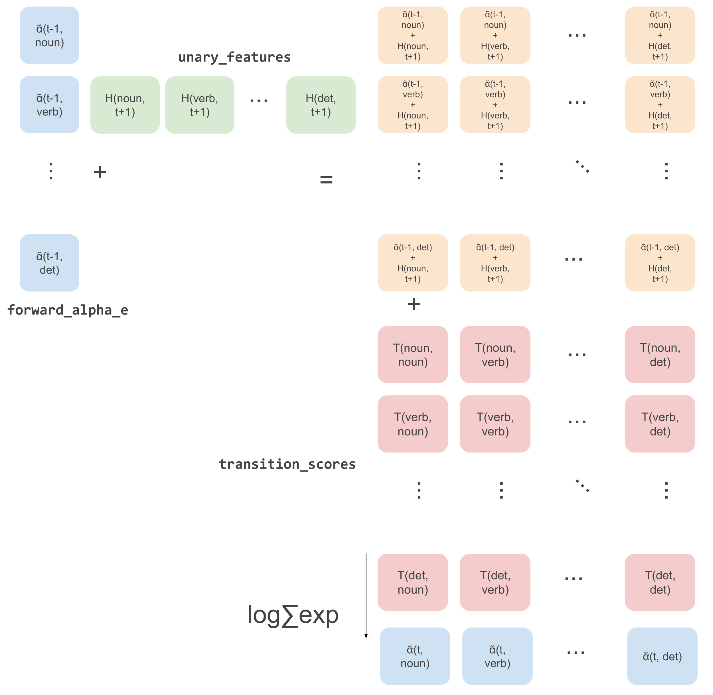
The image above has \(\tilde{\alpha}\) which should be \(\hat{\alpha}\) actually but I can’t for the life of me
figure out how to do that in Google drawings >:(.
Note that we add the transition from each tag to the final <EOS> tag outside of the loop over time, because these are independent
of time and should happen for every sequence in the batch. Then the whole function returns:
logsumexp(alphas) which is \(Z(\mathbf{x}) = \sum_{y^{\prime}_m}\hat{\alpha}(m-1, y^{\prime}_m)\).
This is possible for all examples in the batch because we make sure within the loop over time to only update the alphas
for the sequences that haven’t ended yet. Whenever the value for a particular time-step of the input_mask is zero,
the following lines of code make sure that we retain the old alpha for those examples:
forward_alpha = (
        logsumexp(next_forward_alpha, 1) * input_mask[time].view(batch_size, 1)
        + forward_alpha * (1 - input_mask[time]).view(batch_size, 1)
)
Yay, that’s calculating the partition function! Now let’s look at calculating the nominator of the CRF,
or the function ChainCRF.score_sentence(...).
Calculating the Nominator
To finish calculating the loss, we just need to calculate the (log-)nominator.
\[\sum_{t=1}^m \underbrace{\boldsymbol{\theta}_1 f(y_t^{(i)}, \mathbf{x}^{(i)}, t)}_{\text{unary_features}} + \sum_{t=1}^{m-1} \underbrace{\boldsymbol{\theta}_2 f(y_t^{(i)}, y_{t+1}^{(i)})}_{\text{transition_scores}}\]Which is simply a sum over time of the unary features and the transition probabilities for a given input sentence \(\mathbf{x}^{(i)}\)
and target tag sequence \(\mathbf{y}^{(i)}\). In the implementation we loop over all the sequences in the batch in parallel,
get the current tag for each example in the batch from the ground-truth sequence target_tags,
and calculate the current unary scores and transition scores from the current time to the next.
def score_sentence(self, input_features: torch.Tensor,
                   target_tags: torch.Tensor,
                   input_mask: torch.Tensor) -> torch.Tensor:
        """
        Calculates the log-nominator of the CRF for given batch of
        input features and sequences of target tags.
        :param input_features: the features for each input sequence
            [batch_size, sequence_length, num_tags]
        :param target_tags: tensor with the ground-truth target tags
            of size [batch_size, sequence_length]
        :param input_mask: the binary mask determining which of the input
            entries are padding [batch_size, sequence_length]

        Returns: the log-nominator of the CRF [batch_size]
        """
        batch_size, sequence_length, num_tags = input_features.size()

        # Make time major, for the loop over time.
        input_features = input_features.transpose(0, 1)
        # input_features: [sequence_length, batch_size, num_tags]
        input_mask = input_mask.float().transpose(0, 1)
        # input_mask: [sequence_length, batch_size]
        target_tags = target_tags.transpose(0, 1)
        # target_tags: [sequence_length, batch_size]

        # Get tensor of root tokens and tensor of next tags (first tags).
        root_tags = torch.LongTensor([self.root_idx] * batch_size)
        if torch.cuda.is_available():
          root_tags.to(device)
        next_tags = target_tags[0].squeeze()

        # Initial transition is from root token to first tags.
        initial_transition = self.log_transitions[root_tags, next_tags]

        # Initialize scores.
        scores = initial_transition
        # scores: [batch_size]

        # Loop over time and at each time calculate the score from t to t + 1.
        for time in range(sequence_length - 1):

            # Calculate the score for the current time step.
            unary_features = input_features[time]
            # unary_features: [batch_size, num_tags]
            next_tags = target_tags[time + 1].squeeze()
            current_tags = target_tags[time].squeeze(dim=1)
            unary_features = torch.gather(unary_features, 1,
                                          current_tags.unsqueeze(1)).squeeze()
            # unary_features: [batch_size]
            transition_scores = self.log_transitions[current_tags, next_tags]
            # transition_scores: [batch_size]

            # Add scores.
            scores = scores + transition_scores * input_mask[time + 1]
                        + unary_features * input_mask[time]
            # scores: [batch_size]

        # Gather the last tag for each example in the batch.
        last_tag_index = input_mask.sum(0).long() - 1
        last_tags = torch.gather(target_tags,
                                 0,
                                 last_tag_index.view(1, batch_size)).view(-1)

        # Get the transition scores from the last tag to the <EOS> tag.
        end_tags = torch.LongTensor([self.end_idx] * batch_size)
        if torch.cuda.is_available():
            end_tags = end_tags.to(device)
        last_transition = self.log_transitions[last_tags, end_tags]

        # Add the last input if its not masked.
        last_inputs = input_features[-1]
        last_input_score = last_inputs.gather(1, last_tags.view(-1, 1))
        last_input_score = last_input_score.squeeze()

        scores = scores + last_transition + last_input_score * input_mask[-1]
        return scores
In the code above we calculate the unary features for the tags at the current time step with the following line:
unary_features = torch.gather(unary_features,
                              1,
                              current_tags.unsqueeze(1)).squeeze()
Here, current_tags is a vector with the index of the tag at time \(t\) in the sequence for each example in the batch,
and the gather function retrieves this index in the first dimension of the vector unary_features, which is of size
[batch_size, num_tags], meaning this code gathers \(\boldsymbol{\theta}_1 f(y_t^{(i)}, \mathbf{x}^{(i)}, t)\)
for all examples in the batch. Then we add these unary features to the transition features for each current tag to
the next tags at time \(t+1\) (\(\boldsymbol{\theta}_2 f(y_t^{(i)}, y_{t+1}^{(i)})\)), making sure to mask any
unary features for sequences that have ended, and transition scores for sequences that don’t have a tag anymore at time
\(t+1\):
scores = scores + transition_scores * input_mask[time + 1]
                        + unary_features * input_mask[time]
Then outside of the loop over time we still need to gather the transition scores for the last tag of each sequence in the batch
to the <EOS> token, because we didn’t do this inside the loop. Additionally, we need to add the last unary features for
the longest sequences in the batch. Finally, we return a log-nominator score for each sequence in the batch.
This concludes the calculation of the NLL! So we can start decoding.
Viterbi Decoding
We’ll finally implement decoding with Viterbi. Recall that in structured prediction we ideally want to use an efficient DP algorithm, to get rid of the exponential decoding complexity. As mentioned, decoding here is finding the maximum scoring target sequence according to our model. This amounts to solving the following equation:
\(\mathbf{y}^{\star} = arg\max_{\mathbf{y} \in \mathcal{Y}} p(\mathbf{y} \mid \mathbf{x})\).
With Viterbi, the time complexity of doing this is \(m \cdot |S|^2\), instead of \(|S|^m\) if done naively. Viterbi works very similarly to BP, but instead of summing we maximize. The Viterbi implementation is by far the most complex one of all the CRF methods, especially in the batched version that we’ll use. It’s also the longest function as we have to implement both the forward recursion to calculate all the likelihoods of the possible sequences, as well as backtracking by following backpointers to obtain the maximum scoring sequence, so we’ll do it in two steps. That said, if you went through forward belief propagation and understood that part, this is not much different.
The recursion equations for Viterbi decoding are four equations, one for initializing the recursion variables, one for the recursion itself, one for intializing the backpointers and one for recursively finding the backpointer. If you want a detailed explanation of how we get to these equations from the \(arg\max\) above, see part one of this series
\[\begin{aligned} v(1, y^{\prime}_2) &= \max_{y^{\prime}_1}\psi(y^{\prime}_1, \mathbf{x}, 1) \cdot \psi(y^{\prime}_1, y^{\prime}_{2}) \\ v(t, y^{\prime}_{t+1}) &\leftarrow \max_{y^{\prime}_{t}}\psi(y^{\prime}_t, \mathbf{x}, t) \cdot \psi(y^{\prime}_t, y^{\prime}_{t+1})\cdot v(t-1, y^{\prime}_t) \\ \overleftarrow{v}(1, y^{\prime}_2) &= arg\max_{y^{\prime}_1}\psi(y^{\prime}_1, \mathbf{x}, 1) \cdot \psi(y^{\prime}_1, y^{\prime}_{2}) \\ \overleftarrow{v}(t, y^{\prime}_{t+1}) &\leftarrow arg\max_{y^{\prime}_{t}}\psi(y^{\prime}_t, \mathbf{x}, t) \cdot \psi(y^{\prime}_t, y^{\prime}_{t+1})\cdot v(t-1, y^{\prime}_t) \\ \end{aligned}\]The animation that graphically depict what goes on in Viterbi is the following:
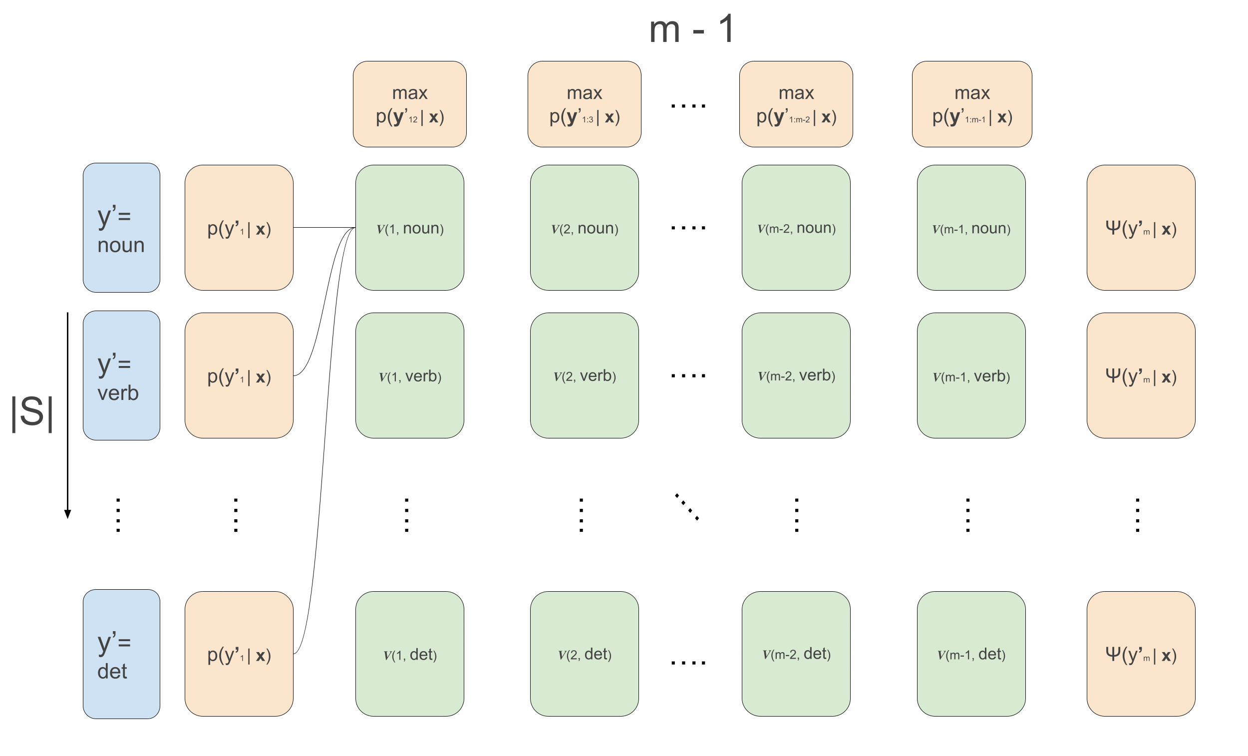
We loop over the sequence, calculating the recursion for each example in the batch and for each tag \(y_t\), and at the same time we keep track for each tag which previous tag is the argument that maximizes the sequence up till that tag. This is what the first loop over time in the code below does. Then, we loop backwards over time and follow the backpointers to find the maximum scoring sequence. The code below implements all this, and below it we’ll go over some more detailed explanations of what’s going, relating the code to the equations. I also write much more detailed comments than usually in the code below for clarification.
Now even though in this code we do need to have an if-else-statement within the loop over time to
keep track of the best last tags (the final column in the above animation). We will still rewrite the recursion
equations like we did above in forward BP to get rid of the need to separately calculate the final recursive calculation
for which we don’t have transition probabilities.
I’m just going to redefine the \(\overleftarrow{v}\) below to avoid notational clutter. Let’s also write everything in logspace while we’re at it.
Note that since \(exp(\cdot)\) and \(\log(\cdot)\) are monotonically increasing functions and we only care about
the maximizing scores and tags, we can just leave them out of the implementation all together. Therefore, in the second line of
equations below for both \(\hat{v}(1, y^{\prime}_2)\) and \(\hat{v}(t, y^{\prime}_{t+1})\) we’ll leave them out, making those equations
formally incorrect, but it doesn’t matter for finding the maximizing sequence. And finally,
note in the below that we assume \(\psi(y^{\prime}_1, \mathbf{x}, 1)\) of the first tag to be 1
because it’s just always the <ROOT> and \(\psi(y^{\prime}_1, y^{\prime}_{2})\) to be the transition probabilities from the root tag to
any other tag. This means the initial \(y^{\prime}_1\) that maximizes the equations is simply <ROOT>.
I annotated the equations with the variables used in the code again, even though in the equations its all for a single example and in the code for a batch of examples. We’re going to do this function in two parts (even though they’re actually a single function), where the first part is the forward recursion given by the above equations and the second part will be backtracking.
def viterbi_decode(self, input_features: torch.Tensor,
                   input_lengths: torch.Tensor):
        """
        Find the maximum scoring tag sequence for each example in the batch.

        :param input_features: the features for each input sequence
            [batch_size, sequence_length, num_tags]
        :param input_lengths: lengths of each example in the batch [batch_size]

        Returns: tuple of scores and tag sequences per example in the batch.
        """
        batch_size, sequence_length, num_tags = input_features.size()

        # We don't have input features for the tags <ROOT> and <EOS>,
        # so we artifially add those at the tag-dimension.
        # See in the class constructor above that the last
        # two indices are for the <ROOT> and <EOS> tags.
        input_features = torch.cat([input_features,
                                   torch.zeros([batch_size,
                                                sequence_length, 2],
                                                device=device) - 10000.],
                                   dim=2)

        # Initialize the viterbi variables in log space
        # and set the score of the root tag the highest.
        init_vit = torch.full((1, self.num_tags), -10000., device=device)
        init_vit[0][self.root_idx] = 0

        # Initialize tensor to keep track of backpointers.
        # This tensor will hold the red arrow backpointers
        # like in the animation above the code.
        backpointers = torch.zeros(batch_size, sequence_length, self.num_tags,
                                   device=device).long() - 1
        # These lists will hold the best last tags and path scores for
        # each example in the batch. I.e., when t equals their sequence length.
        best_last_tags = []
        best_path_scores = []

        # forward_vit at step t holds the viterbi variables for step t - 1
        # will be different for each example in batch, but start the same.
        forward_vit = init_vit.unsqueeze(0).repeat(batch_size, 1, 1)

        # A counter counting down from number of examples in batch to 0.
        num_examples_left = batch_size

        # Loop over the sequence for the forward recursion.
        for t in range(sequence_length):

            # Find the sequences that are ending at this t.
            ending = torch.nonzero(input_lengths == t)
            n_ending = len(ending)

            if n_ending > 0:

                # Get the viterbi vars of the ending sequences.
                # Important here is that the sequences are ordered descending in
                # length. Meaning the last sequences are ending the first.
                forward_ending = forward_vit[
                    (num_examples_left - n_ending):num_examples_left]

                # The terminal var giving the best last tag is
                # the viterbi variables + trans. prob. to end token.
                trans_to_end = self.log_transitions[:, self.end_idx]
                terminal_var = forward_ending + trans_to_end.unsqueeze(0)

                # Get the final best score and tag for these sequences.
                path_scores, best_tag_idx = torch.max(terminal_var, 1)

                # First sequence to end is last sequence in batch, so if
                # we save them like this and reverse the lists
                # later on we get the right ordering back.
                for tag, score in zip(reversed(list(best_tag_idx)),
                                      reversed(list(path_scores))):
                    best_last_tags.append(tag)
                    best_path_scores.append(score)

                # Update counter that tracks how many sequences haven't ended.
                num_examples_left -= n_ending

            # Calculate scores of next tag
            forward_vit = forward_vit.view(batch_size, self.num_tags, 1)
            transition_scores = self.log_transitions.unsqueeze(0)
            next_tag_vit = forward_vit + transition_scores

            # Get the best next tags and viterbi vars.
            viterbivars_t, idx = torch.max(next_tag_vit, 1)
            best_tag_ids = idx.view(batch_size, -1)

            # Get unary scores at current time step.
            unary_features = input_features[:, t, :].view(batch_size,
                                                          self.num_tags, 1)

            # Add the unary features and assign forward_vit to the set
            # of viterbi variables we just computed.
            forward_vit = (viterbivars_t + unary_features.squeeze(2)).view(
                                        batch_size, -1)

            # Save the best tags as backpointers.
            backpointers[:, t, :] = best_tag_ids.long()

        # Get final ending sequences and calculate the best last tags
        ending = torch.nonzero(input_lengths == sequence_length)
        ending = ending.cuda() if torch.cuda.is_available() else ending
        n_ending = len(ending)

        if n_ending > 0:

            forward_ending = forward_vit[
                        (num_examples_left - n_ending):num_examples_left]

            # transition to STOP_TAG
            last_transitions = self.log_transitions[:, self.end_idx].unsqueeze(0)
            terminal_var = forward_ending + last_transitions
            path_scores, best_tag_idx = torch.max(terminal_var, 1)

            for tag, score in zip(reversed(list(best_tag_idx)),
                                  reversed(list(path_scores))):
                best_last_tags.append(tag)
                best_path_scores.append(score)

        # Backtracking (see code below).
        ...
Everything in the code above hopefully becomes clear with the equations with annotations given above the code.
Below I took out a piece of code that’s inside of the if-statements in the code above. What happens is that we calculate:
\(\hat{y}^{\prime}_m = arg\max_{y^{\prime}_m}\underbrace{\boldsymbol{\theta}_2 f(y^{\prime}_m, y^{\prime}_{m+1})}_{\text{trans_to_end}} + \underbrace{\hat{v}_{m-1}(y^{\prime}_m)}_{\text{forward_ending}}\),
for every example that is ending at that time \(t\), i.e., \(t = m\), and for \(y^{\prime}_{m+1}\) the <EOS>-tag.
if n_ending > 0:

        # Get the viterbi vars of the ending sequences.
        # Important here is that the sequences are ordered descending in
        # length. Meaning the last sequences are ending the first.
        forward_ending = forward_vit[
            (num_examples_left - n_ending):num_examples_left]

        # The terminal var giving the best last tag is
        # the viterbi variables + trans. prob. to end token.
        trans_to_end = self.log_transitions[:, self.end_idx]
        terminal_var = forward_ending + trans_to_end.unsqueeze(0)

        # Get the final best score and tag for these seequences.
        path_scores, best_tag_idx = torch.max(terminal_var, 1)

        # First sequence to end is last sequence in batch, so if
        # we save them like this and reverse the lists
        # later on we get the right ordering back.
        for tag, score in zip(reversed(list(best_tag_idx)),
                              reversed(list(path_scores))):
            best_last_tags.append(tag)
            best_path_scores.append(score)

        # Update counter that tracks how many sequences haven't ended.
        num_examples_left -= n_ending
We do the same calculation outside of the loop over time for all the sequences that have the maximum sequence length
in the batch. Then at the end of the loop we have all the backpointers and scores initialized, and we can start the backtracking.
In the lists best_last_tags we appended the final tags that maximized the ending sequences, starting with the shortest
sequences in the batch. When we make sure to sort all the sequences in the batch in descending order,
we can simply reverse best_last_tags to get the original ordering back. In the code below, we then put these tags in the initialized
matrix best_paths that should hold the maximizing sequence for each example. This means best_paths looks like the image below before we loop backwards over time:
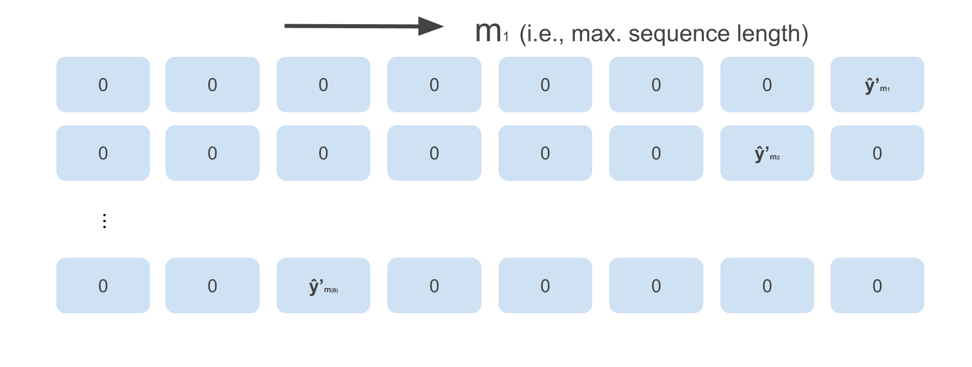
(just an example, depending on how long each sequence in the batch is the actual batch might look differently).
Then we loop backwards over time, following the backpointers, and fill the best_paths for each time in the sequence.
def viterbi_decode(self, input_features: torch.Tensor,
                   input_lengths: torch.Tensor):
        """
        Find the maximum scoring tag sequence for each example in the batch.

        :param input_features: the features for each input sequence
            [batch_size, sequence_length, num_tags]
        :param target_tags:
        :param input_lengths: lengths of each example in the batch [batch_size]

        Returns: tuple of scores and tag sequences per example in the batch.
        """

        # Forward Recursion (see code above).
        ...

        # Reverse the best last tags (and scores) to get the original order.
        best_last_tags = torch.LongTensor(list(reversed(best_last_tags)))
        if torch.cuda.is_available()
            best_last_tags = best_last_tags.cuda()
        best_path_scores = torch.LongTensor(list(reversed(best_path_scores)))
        if torch.cuda.is_available():
            best_path_scores = best_path_scores.cuda()

        # Initialize the best paths for each sequence in the batch by
        # putting at the correct length for each example
        # the best last tag found in the above recursion.
        # This is depicted in the image above.
        best_paths = torch.zeros(batch_size, sequence_length + 1).long()
        if torch.cuda.is_available():
            best_paths = best_paths.cuda()
        best_paths = best_paths.index_put_(
            (torch.LongTensor([i for i in range(backpointers.size(0))]),
             input_lengths),
            best_last_tags)

        # A counter keeping track of number of active sequences.
        # This increases from 0 until batch_size at the last time step
        # when even the shortest sequence is active.
        num_active = 0

        # Loop backwards over time (max. time to 0).
        for t in range(sequence_length - 1, -1, -1):

            # If time step equals lengths of some sequences, they are starting.
            # (starting meaning this time step is their last tag).
            starting = torch.nonzero(input_lengths - 1 == t)
            n_starting = len(starting)

            # If there are sequences starting, grab their best last tags.
            if n_starting > 0:
                # For the longest sequences, initialize best_tag_id.
                if t == sequence_length - 1:
                    best_tag_id = best_paths[num_active:num_active + n_starting,
                                             t + 1]
                else:
                    last_tags = best_paths[num_active:num_active + n_starting,
                                           t + 1]
                    best_tag_id = torch.cat((best_tag_id,
                                             last_tags.unsqueeze(1)), dim=0)

                # Update the number of active sequences.
                num_active += n_starting

            # Get relevant backpointers based on sequences that are active.
            active = backpointers[:num_active, t]

            # Follow the backpointers to the best previous tag.
            best_tag_id = best_tag_id.view(num_active, 1)
            best_tag_id = torch.gather(active, 1, best_tag_id)
            best_paths[:num_active, t] = best_tag_id.squeeze()

        # Sanity check that first tag is the <ROOT> token.
        assert (best_paths[:, 0].sum().item() \
                    == best_paths.size(0) * self.root_idx)

        # Return the scores and the paths without the <ROOT> token.
        return best_path_scores, best_paths[:, 1:]
In the above code, at every time step (for the active sequences) we use the previous best tags, starting with
the best last tags, to find the correct backpointer to follow back. Now backpointers is a matrix of size [batch_size, sequence_length, num_tags] (where
the batch is still sorted in descending order) and holds at every time \(t\) the backpointers (i.e., ids of previous tags
that maximize the sequence) for every tag. See this for one example in a batch depicted below:
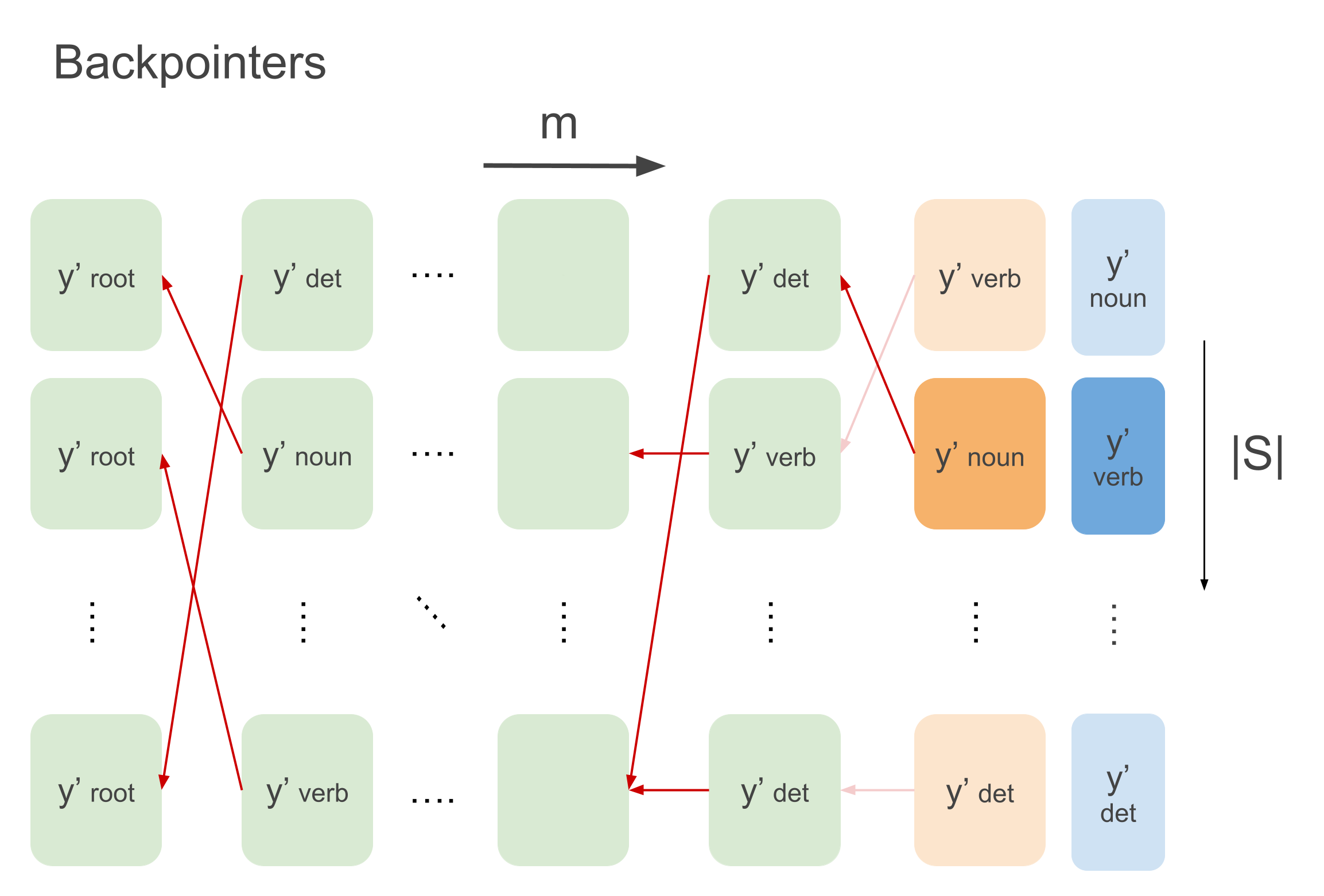
Now best_last_tags holds the tag to start backtracking with for every example, which might be a verb like depicted above.
Based on this last tag you just need to follow the path backward to find the correct sequence. Selecting the backpointer
is what happens in the following lines (where active holds the backpointers for the active sequences):
# Follow the backpointers to the best previous tag.
best_tag_id = best_tag_id.view(num_active, 1)
best_tag_id = torch.gather(active, 1, best_tag_id)
best_paths[:num_active, t] = best_tag_id.squeeze()
In the end, best_paths holds the maximizing sequence for every example in the batch, starting at the <ROOT> tag.
We return the scores and the sequences without the root and we are done!
Summarizing
We’ve implemented all the methods needed for a bi-LSTM-CRF POS tagger! We’ve taken care of batched forward belief propagation and calculating the nominator, together forming our loss function. Then we implemented Viterbi decoding to find the predicted tag sequence with maximum probability. Now, we only need to get some data and train our model on it. Go to part three to train this model on real POS tagging data!
Sources
Xuezhe Ma and Eduard H. Hovy. 2016. End-to-end sequence labeling via bi-directional LSTM-CNN-CRF. In ACL.
Matt Gardner and Joel Grus and Mark Neumann and Oyvind Tafjord and Pradeep Dasigi and Nelson F. Liu and Matthew Peters and Michael Schmitz and Luke S. Zettlemoyer. 2017 AllenNLP: A Deep Semantic Natural Language Processing Platform.