Structured Prediction part one - Deriving a Linear-chain CRF

You’re looking at part one of a series of posts about structured prediction with conditional random fields. In this post, we’ll talk about linear-chain CRFs applied to part-of-speech (POS) tagging. In POS tagging, we label all words with a particular class, like verb or noun. This can be useful for things like word-sense disambiguation, dependency parsing, machine translation, and other NLP applications. In the following, we will cover the necessary background to understand the motivation behind using a CRF, talking about things like discriminative and generative modeling, probabilistic graphical models, training a linear-chain CRF with efficient inference methods using dynamic programming like belief propagation (AKA the forward-backward algorithm), and decoding with Viterbi. In part two, we will implement all these ingredients in the popular deep learning library PyTorch. If you want to skip the background and start implementing, go to part two, where we’ll put a linear-chain CRF on top of a bidirectional LSTM and in part three train it all end-to-end on a POS tagging dataset. OK! Let’s start.

Consider the following sentence that is partly annotated with POS tags:

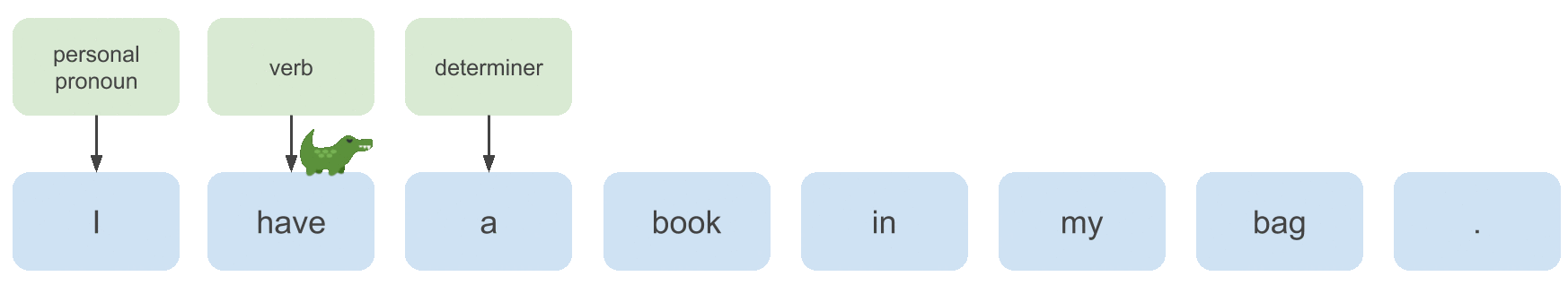
Whether the POS tag we want to continue the labeling process with here is a noun or a verb depends on the POS tag of the previous word. In this case the previous label is determiner, so we want to choose noun. For sequence labeling tasks like this, and more general for structured prediction tasks, it is helpful to model the dependencies among the labels.

Structured Prediction

Structured prediction is a framework for solving problems of classification or regression in which the output variables are mutually dependent or constrained. It can be seen as a subset of prediction where we make use of the structure in the output space. The loss function used in structured prediction problems considers the outputs as a whole.

Let’s denote the input sequence of words by \(\mathbf{x}\), the output space (i.e., the set of all possible target sequences) by \(\mathcal{Y}\) and \(f(\mathbf{x}, \mathbf{y})\) some function that expresses how well \(\mathbf{y}\) fits \(\mathbf{x}\) (we will clarify what this function is later), then prediction can be denoted by the following equation:

\[\mathbf{y}^{\star} = arg \max_{\mathbf{y} \in \mathcal{Y}} f(\mathbf{x}, \mathbf{y})\]

The reason that we distinguish structured prediction from regular classification is that for the former the search that needs to be done over the output space – finding the \(\mathbf{y} \in \mathcal{Y}\) that maximizes the function \(f(\mathbf{x}, \mathbf{y})\) – is usually intractable. To see why, assume that the number of possible POS tags is \(|\mathcal{S}|\) and the sequence length \(m\), then there are \(|\mathcal{S}|^m\) possible sequences we would need to search over. This motivates the use of efficient inference and search algorithms. Note that if we would ignore the dependencies in the output space and simply proceed decoding ‘greedily’, we could use the following formula for prediction for all words in the input sequence separately, requiring only \(|\mathcal{S}|\cdot m\) operations:

\[y_i^{\star} = arg \max_{y \in \mathcal{S}} f(\mathbf{x}, y_i, i) \text{ for } i \in \{1, \dots, m\}\]

Conditional Random Field

A conditional random field (CRF, Lafferty et al., 2001) is a probabilistic graphical model that combines advantages of discriminative classification and graphical models.

Discriminative vs. Generative models

In the discriminative approach to classification we model \(p(y \mid x)\) directly as opposed to the generative case where we model \(p(x \mid y)\) and use it together with Bayes’ rule for prediction. If we model the conditional directly, dependencies among \(x\) itself play no rule, resulting in a much simpler inference problem than modeling the joint \(p(y, x)\). Generative models describe how some label \(y\) can generate some feature vector \(x\), whereas discriminative models directly describe how to assign a feature vector \(x\) a label \(y\). CRFs are discriminative models.

Graphical Models

Probabilistic graphical models (PGMs) represent complex distributions over many variables as a product of local factors of smaller subsets of variables. Generative models are often most naturally represented by directed graphical models (because they assume Y generates X, \(p(x,y) = p(y)p(x \mid y)\)), whereas discriminative models are most naturally represented by undirected graphical models (models \(p(y \mid x)\) directly). See in the figure below a generative PGM on the left, and a discriminative on the right.

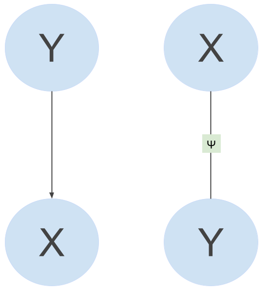
CRFs are discriminative models and can be represented as factor graphs. A factor graph is an undirected graph \(G = (V,F,E)\), in which \(V\) denotes the random variables (the blue circles in the image above), \(F\) denotes the factors (the green square between the variables in the image above), and \(E\) the edges. A factor graph describes how a complex probability distribution factorizes, and thus imposes independence relations. A distribution \(p(\mathbf{y})\) factorizes according to a factor graph \(G\) if there exists a set of local functions \(\psi_a\) such that \(p\) can be written as:

\[p(\mathbf{y}) = \frac{1}{Z} \prod_{a \in F} \psi_a(y_{N(a)})\]

The factors \(\psi_a\) are each only dependent on the neighbors \(y_i\) of \(a\) (denoted by \(y_{N(a)}\)) in the factor graph. For example, \(N(a)\) for \(\psi_a\) in the image above ar \(X\) and \(Y\). The factors have to be larger than zero, and \(Z\) makes sure the whole thing is normalized (sums to 1). Based on what kind of graphical structure (i.e., conditional independence assumptions) one assumes, one can use linear chain CRFs or more general CRFs. Because we want each POS tag to depend on the previous tag, we use a linear-chain CRF.

Linear-Chain CRF

Now it’s time to design a CRF for POS tagging. We will use the fact that we want the prediction for each tag \(y_i\) to depend on both the previously predicted tag \(y_{i-1}\) and the input sequence of words \(\mathbf{x}\). This gives us the following factor graph:

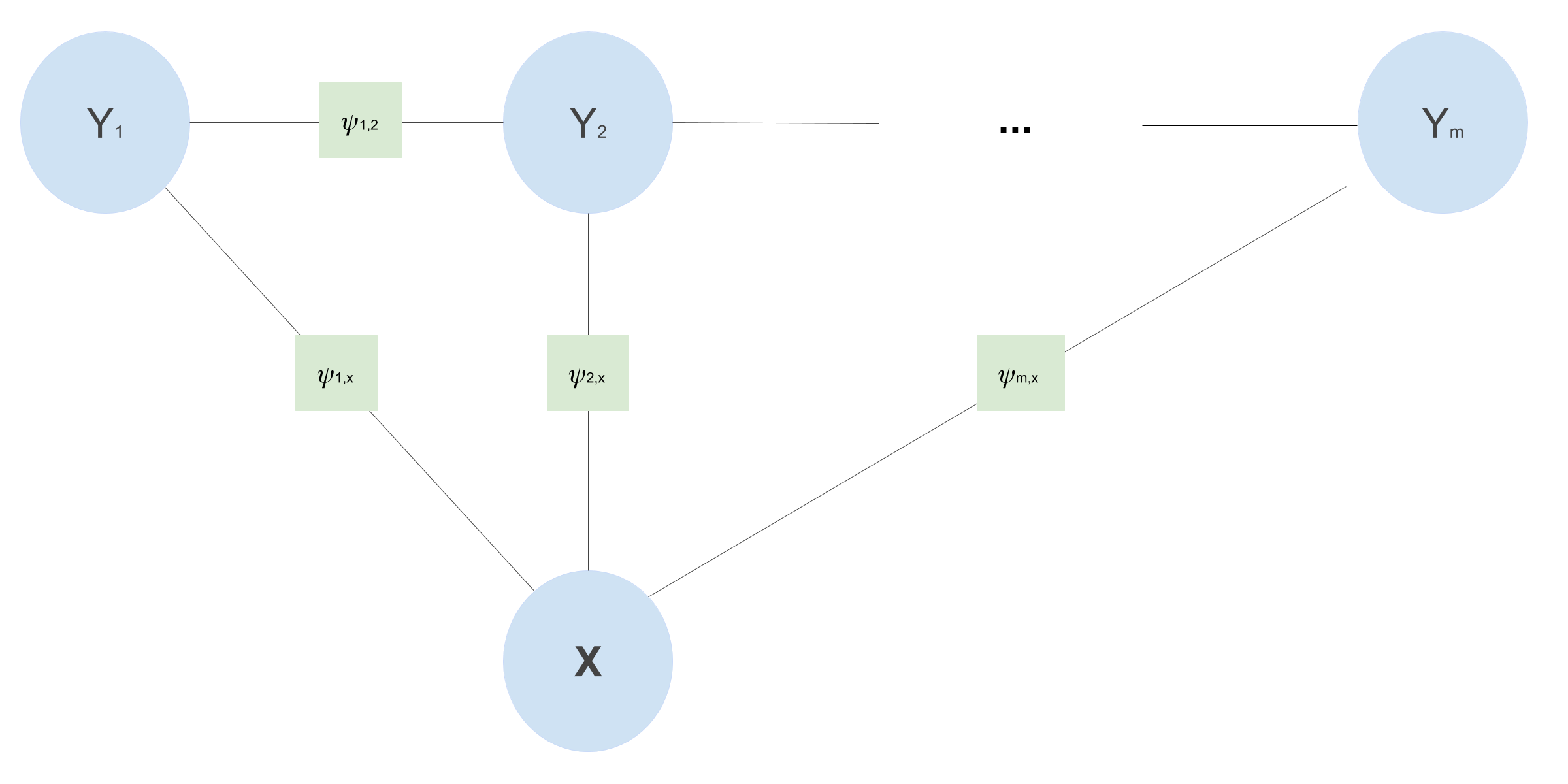
This particular linear-chain CRF implies the following conditional independence assumptions:

• Each POS tag is only dependent on its immediate predecessor and successor and \(\mathbf{x}\): \(y_t \mathrel{\unicode{x2AEB}} \{y_1, \dots, y_{t - 2}, y_{t + 2}, \dots, y_m\} \mid y_{t - 1}, y_{t + 1}, \mathbf{x}\)

We can simply multiply all the factors in the above factor graph to get our the factorized conditional probability distribution:

\[\begin{aligned} p(\mathbf{y} \mid \mathbf{x}) &= \frac{1}{Z(\mathbf{x})} \prod_{t=1}^{m} \psi(y_t, \mathbf{x}, t) \prod_{t=1}^{m-1}\psi(y_t, y_{t+1}) \\ \end{aligned}\]

Additionally, what makes a CRF a CRF is that it’s simply a specific way of choosing the factors, or in other words feature functions. The CRF-way of defining the factors is taking an exponential of a linear combination of real-valued feature functions \(f(\cdot)\) with parameters \(\boldsymbol{\theta}_1\) and \(\boldsymbol{\theta}_2\). You’ll see in the following that the feature functions and parameters are shared over timesteps:

\[\begin{aligned} p(\mathbf{y} \mid \mathbf{x}) &= \frac{1}{Z(\mathbf{x})} \prod_{t=1}^{m} \exp\left(\boldsymbol{\theta}_1 \cdot f(y_t, \mathbf{x}, t)\right)\prod_{t=1}^{m-1} \exp\left(\boldsymbol{\theta}_2 \cdot f(y_t, y_{t+1})\right) \\ &= \frac{1}{Z(\mathbf{x})} \exp\left(\sum_{t=1}^m \boldsymbol{\theta}_1 \cdot f(y_t, \mathbf{x}, t) + \sum_{t=1}^{m-1} \boldsymbol{\theta}_2 \cdot f(y_t, y_{t+1})\right) \\ Z(\mathbf{x}) &= \sum_{\mathbf{y}^{\prime}}\exp\left(\sum_{t=1}^m \boldsymbol{\theta}_1 \cdot f(y^{\prime}_t, \mathbf{x}, t) + \sum_{t=1}^{m-1} \boldsymbol{\theta}_2 \cdot f(y^{\prime}_t, y^{\prime}_{t+1})\right) \end{aligned}\]

Intuitively, the first sum in the exponent above should represent the probabilities that a particular \(y_t\) is the right POS tag at time \(t\), and the second sum should represent the probabilities that each \(y_{t+1}\) follows a particular \(y_{t}\). Luckily, we don’t need to hand-engineer the feature functions to reflect these intuitions anymore and can hit it with the DL hammer :) (which we will cover in part two of this series). The value \(Z(\mathbf{x})\) is just the partition function ensuring that this formula is a properly defined probability distribution that sums to 1. Again, here the sum over all possible sequences of \(\mathbf{y}\) appears, and naive methods of computing this sum are intractable, which is why we will use belief propagation!

Training a Linear-Chain CRF

We can train the CRF with regular maximum likehood estimation, given a set of \(N\) datapoints. Performing gradient descent over the likelihood will require computing the factors from the PGM, which can be efficiently found with probabilistic inference methods like belief propagation. Let’s take a look at the log-likelihood:

\[\begin{aligned} \log \mathcal{L}(\boldsymbol{\theta}) &= \log{\prod_{i=1}^N p(\mathbf{y}^{(i)} \mid \mathbf{x}^{(i)}, \boldsymbol{\theta}) } = \log{\Bigg[\prod_{i=1}^N \frac{1}{Z(\mathbf{x}^{(i)})}\prod_{t=1}^m \psi (y_t^{(i)}, \mathbf{x}_t^{(i)}, t) \prod_{t=1}^{m-1} \psi (y_t^{(i)}, y_{t+1}^{(i)}) \Bigg]} \\ &= \log{\Bigg[\prod_{i=1}^N \frac{1}{Z(\mathbf{x}^{(i)})} \exp\Bigg(\sum_{t=1}^m \boldsymbol{\theta}_1 f(y_t^{(i)}, \mathbf{x}_t^{(i)}, t) + \sum_{t=1}^{m-1} \boldsymbol{\theta}_2 f(y_t^{(i)}, y_{t+1}^{(i)})\Bigg)\Bigg]} \\ &= \log{\Bigg[\prod_{i=1}^N \exp\Bigg(\sum_{t=1}^m \boldsymbol{\theta}_1 f(y_t^{(i)}, \mathbf{x}_t^{(i)}, t) + \sum_{t=1}^{m-1} \boldsymbol{\theta}_2 f(y_t^{(i)}, y_{t+1}^{(i)})\Bigg)\Bigg]} + \log{\Bigg[\prod_{i=1}^N \frac{1}{Z(\mathbf{x}^{(i)})} \Bigg]} \\ &= \sum_{i=1}^{N}\sum_{t=1}^m \boldsymbol{\theta}_1 f(y_t^{(i)}, \mathbf{x}_t^{(i)}, t) + \sum_{t=1}^{m-1} \boldsymbol{\theta}_2 f(y_t^{(i)}, y_{t+1}^{(i)}) - \sum_{i=1}^{N}\log\left(Z(\mathbf{x}^{(i)})\right) \\ \end{aligned}\]

To optimize the parameters, we need to calculate the gradients of the log-likelihood w.r.t. the parameters:

\[\begin{aligned} \nabla_{\boldsymbol{\theta}_1} \log \mathcal{L}(\boldsymbol{\theta}) &= \sum_{i=1}^{N}\sum_{t=1}^m f(y_t^{(i)}, \mathbf{x}_t^{(i)}, t) - \sum_{i=1}^N \nabla_{\boldsymbol{\theta}_1} \log(Z(\mathbf{x}^{(i)})) \\ \nabla_{\boldsymbol{\theta}_1} \log(Z(\mathbf{x}^{(i)})) &= \frac{\nabla_{\boldsymbol{\theta}_1}Z(\mathbf{x}^{(i)})}{Z(\mathbf{x}^{(i)})} \\ &= \frac{\sum_{\mathbf{y}^{\prime}}\exp\left(\sum_{t=1}^m \boldsymbol{\theta}_1 \cdot f(y^{\prime(i)}_t, \mathbf{x}^{(i)}, t) + \sum_{t=1}^{m-1} \boldsymbol{\theta}_2 \cdot f(y^{\prime(i)}_t, y^{\prime(i)}_{t+1})\right) \cdot \sum_{t=1}^m f(y_t^{\prime(i)},\mathbf{x}^{(i)},t)}{Z(\mathbf{x}^{(i)})} \\ &= \sum_{t=1}^m\sum_{y_1^{\prime}}\dots\sum_{y_m^{\prime}} p(\mathbf{y}^{\prime(i)} \mid \mathbf{x}^{(i)}) \cdot f(y_t^{\prime(i)},\mathbf{x}^{(i)},t) \\ &= \sum_{t=1}^m\sum_{y^{\prime}_t} p(y^{\prime(i)}_t \mid \mathbf{x}^{(i)}) \cdot f(y_t^{\prime(i)},\mathbf{x}^{(i)},t) \end{aligned}\]

Where the last step is true because we simply marginalize out all \(y_s\)’s for which \(s \neq t\). Similarly for the gradient w.r.t. \(\boldsymbol{\theta}_2\):

\[\begin{aligned} \nabla_{\boldsymbol{\theta}_2} \log(Z(\mathbf{x}^{(i)})) &= \sum_{t=1}^m\sum_{y^{\prime}_t}\sum_{y^{\prime}_{t+1}} p(y^{\prime(i)}_t,y^{\prime(i)}_{t+1} \mid \mathbf{x}) \cdot f(y_t^{\prime(i)},y_{t+1}^{\prime(i)}) \end{aligned}\]

This shows that for the backward pass over the CRF computations we need the marginals \(p(y_t \mid \mathbf{x})\) and \(p(y_t,y_{t+1} \mid \mathbf{x})\), which we can again compute efficiently with belief propagation.

Efficient Inference with Belief Propagation

For inference we simply need to calculate the function for \(p(\mathbf{y} \mid \mathbf{x})\) for a given input sequence. The nominator is easy to compute, but the denominator requires summing over all possible target sequences, which is intractable. Belief propagation (BP) is an algorithm to do efficient inference in PGMs, and we can use it to get the exponential time for computing the partition function down to polynomial time. Additionally, to calculate the gradients of the log-likelihood w.r.t. the parameters, we need to calculate the marginals. We’ll also use BP for this, but it’s easiest to explain if we first go over how to use it to calculate the partition function.

Recall that, if done naively, the complexity of computing the partition function is \(|S|^m\). With some dynamic programming magic we can use the conditional independence structure to get this down to \(m \cdot |S|^2\). Before I knew dynamic programming the term always sounded difficult to me, but it really is just nothing other than dividing the problem in sub-problems, and identifying which of these sub-problems you are computing more than once. By memorizing the calculations of these sub-problems (memoisation), we can re-use them when we need them again. E.g., if you have a function that calculates \(n!\), you could store the value you calculated when the function is called for \(5!\), and re-use this value when the function is called for \(7! = 5!*6*7\). How we do that in BP can be illustrated well when we write out the sums and products in the partition function (for the sake of this illustration we will use the factors \(\psi(\cdot)\) again):

\[\begin{aligned} Z(\mathbf{x}) &= \sum_{\mathbf{y}^{\prime}}\left(\prod_{t=1}^m \psi(y^{\prime}_t, \mathbf{x}, t) \cdot \prod_{t=1}^{m-1} \psi(y^{\prime}_t, y^{\prime}_{t+1})\right) \\ &= \sum_{y^{\prime}_1}\sum_{y^{\prime}_2}\dots\sum_{y^{\prime}_m}\psi(y^{\prime}_1, \mathbf{x}, 1) \cdot \dots \cdot \psi(y^{\prime}_m, \mathbf{x}, m) \cdot \psi(y^{\prime}_1, y^{\prime}_{2}) \cdot \dots \cdot \psi(y^{\prime}_{m-1}, y^{\prime}_{m}) \end{aligned}\]

Now if we rearrange the sums and take each factor as far forward as possible we get:

\[\begin{aligned} Z(\mathbf{x}) &= \sum_{y^{\prime}_m}\psi(y^{\prime}_m, \mathbf{x}, m)\sum_{y^{\prime}_{m-1}}\psi(y^{\prime}_{m-1}, \mathbf{x}, m-1)\psi(y^{\prime}_{m-1}, y^{\prime}_{m}) \dots \dots \\ & \quad \quad \quad \dots \sum_{y^{\prime}_2}\psi(y^{\prime}_2, \mathbf{x}, 2) \cdot \psi(y^{\prime}_2, y^{\prime}_{3})\underbrace{\sum_{y^{\prime}_1}\psi(y^{\prime}_1, \mathbf{x}, 1) \cdot \psi(y^{\prime}_1, y^{\prime}_{2})}_{\alpha(1, y^{\prime}_{2})} \end{aligned}\]

The above re-arrangement would not be possible if each factor contained all \(y_t\)’s, meaning there would be no conditional independence assumptions (in which case the best conceivable complexity of calculating the partition function is \(|S|^m\)). If we look at the last sum in the above equation, we can view it as a function of \(y^{\prime}_2\): \(\alpha(1, y^{\prime}_2)\), which for each value of \(y^{\prime}_2\) returns the sum over all \(y_1^{\prime}\):

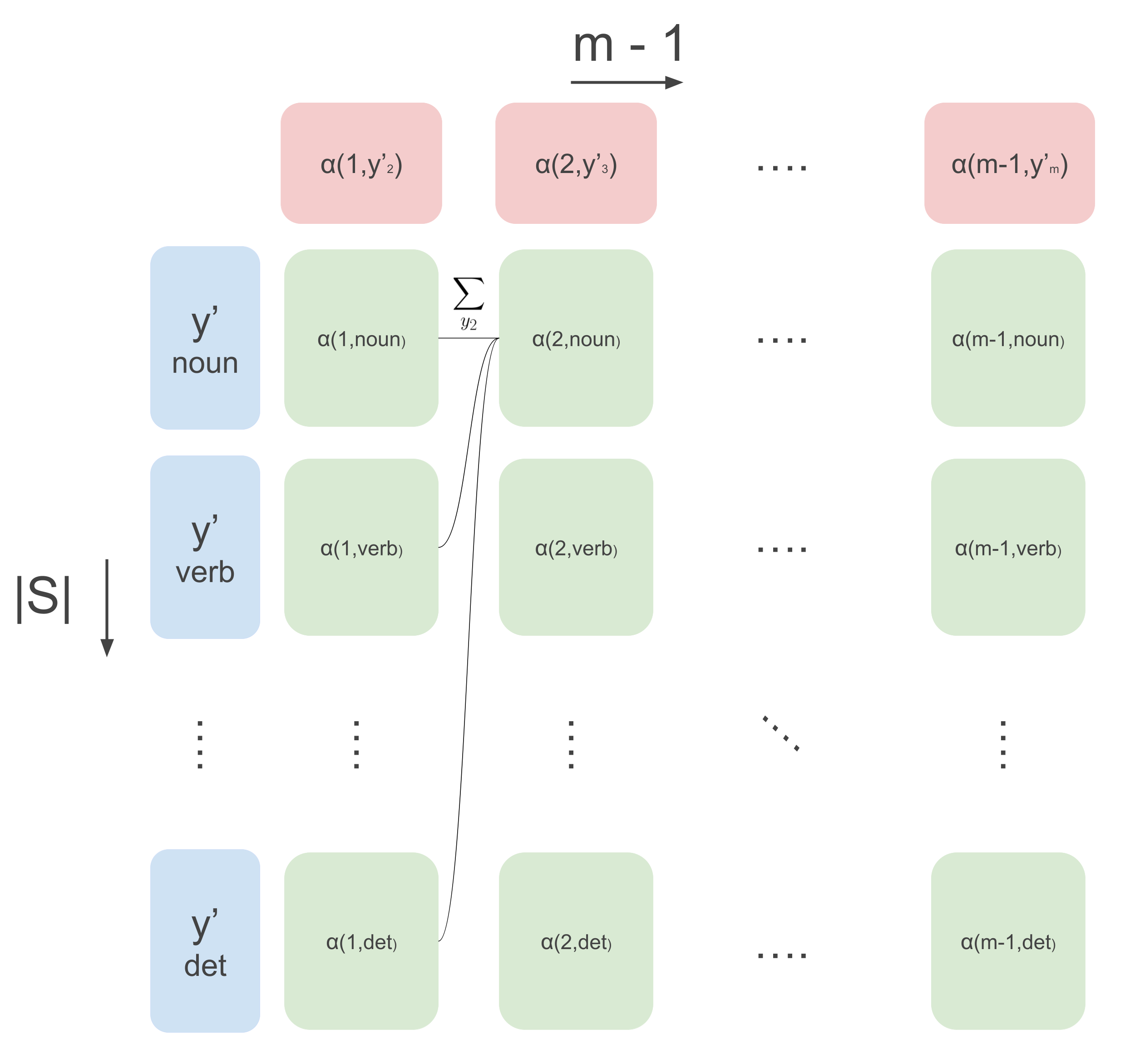
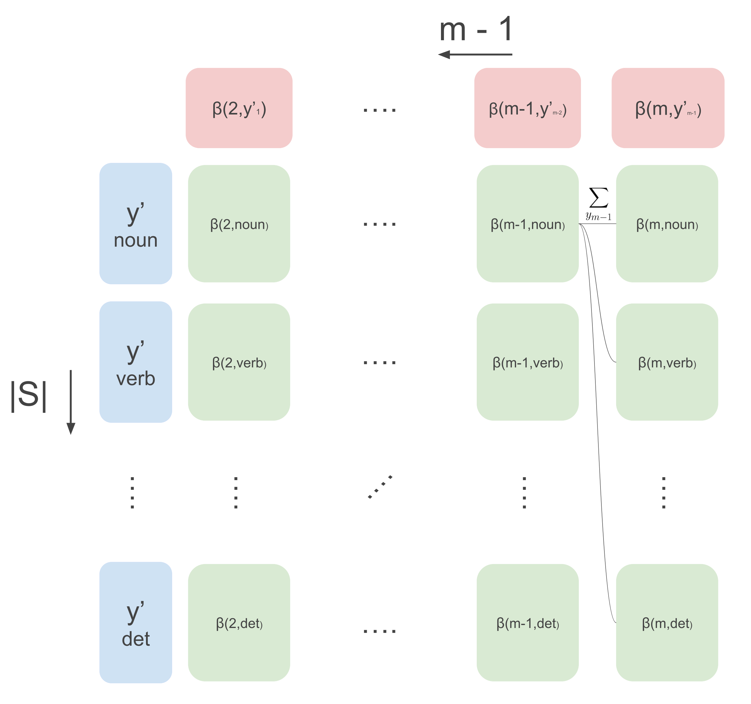
\[\alpha(1, y^{\prime}_2) = \sum_{y^{\prime}_1}\psi(y^{\prime}_1, \mathbf{x}, 1) \cdot \psi(y^{\prime}_1, y^{\prime}_{2})\]

This function can also be seen as a vector of size \(|S|\) (that’s how many values \(y^{\prime}_2\) can take), where each entry represents a sum over, again, \(|S|\) values of \(y^{\prime}_1\) (now we can start to see where the \(|S|^2\) term in the time complexity comes from). We can compute these and use them for the next sum in the equation. Let’s make this a bit clearer with an image. The below image shows the flow of computation in a the DP algorithm belief-propagation. The columns are steps over time (from 1 to \(m-1\)), and the rows are all different values \(y^{\prime}\) can take, which in this case are the POS tags. So the vector representing \(\alpha(1, y^{\prime}_2)\) in the image below is the first column of green boxes. Then for all next time steps we can use the following recursion:

\[\alpha(t, y^{\prime}_{t+1}) \leftarrow \sum_{y^{\prime}_{t}}\psi(y^{\prime}_t, \mathbf{x}, t) \cdot \psi(y^{\prime}_t, y^{\prime}_{t+1})\cdot \alpha(t-1, y^{\prime}_t)\]

So for each green box in the image below, we compute the above recursive function that uses all green boxes from the previous column. This costs \(|S|\) operations for one green box, and we do this for each green box, in total \(|S|^2\) times. We do this for each column, giving us \((m-2) \cdot |S|^2\) operations. If we then also consider the initialization computation for \(\alpha(1, y^{\prime}_2)\) costing \(|S|^2\) operations we get the complexity of \((m - 1) \cdot |S|^2\). And then we just need to calculate the partition function from this, costing another \(|S|^2\) operations (see text below image).

By computing all the column vectors, we can finally get the partition function as follows:

\[Z(\mathbf{x}) = \sum_{y^{\prime}_m}\psi(y^{\prime}_m, \mathbf{x}, m) \cdot\alpha(m-1, y^{\prime}_m)\]

Where \(\alpha(m-1, y^{\prime}_m)\) are the values of the rightmost column. And, we get to the final complexity of \(m \cdot |S|^2\) for computing the partition function. If this is all we wanted, we would be done now. However we also need the marginals for calculating the gradient.

From probability theory we know that computing the marginals from a joint means summing (in the discrete case) over all other variables, to marginalize them out. We need both \(p(y_t \mid \mathbf{x})\) and \(p(y_t, y_{t+1} \mid \mathbf{x})\):

\[\begin{aligned} p(y_t \mid \mathbf{x}) &= \sum_{y_1}\dots\sum_{y_{t-1}}\sum_{y_{t+1}}\dots\sum_{y_m}p(\mathbf{y} \mid \mathbf{x}) \\ p(y_t, y_{t+1} \mid \mathbf{x}) &= \sum_{y_1}\dots\sum_{y_{t-1}}\sum_{y_{t+2}}\dots\sum_{y_m}p(\mathbf{y} \mid \mathbf{x}) \end{aligned}\]

In the previous we saw how to compute this sum if we were to sum over all \(y_t\)’s, but we can also use it to compute the marginals. To this end, we first do the exact same as before to calculate the partition function, but rearranging the sums in a different way:

\[\begin{aligned} Z(\mathbf{x}) &= \sum_{y^{\prime}_1}\psi(y^{\prime}_1, \mathbf{x}, 1)\sum_{y^{\prime}_{2}}\psi(y^{\prime}_{2}, \mathbf{x}, 2)\psi(y^{\prime}_{1}, y^{\prime}_{2}) \dots \dots \\ & \quad \quad \quad \dots \sum_{y^{\prime}_{m-1}}\psi(y^{\prime}_{m-1}, \mathbf{x}, m-1) \cdot \psi(y^{\prime}_{m-1}, y^{\prime}_{m-2})\underbrace{\sum_{y^{\prime}_m}\psi(y^{\prime}_m, \mathbf{x}, m) \cdot \psi(y^{\prime}_{m-1}, y^{\prime}_{m})}_{\beta(m, y^{\prime}_{m-1})} \end{aligned}\]

Now, by similar argument as the forward-case, we can do DP as illustrated by the following image.

We can calculate the rightmost column as follows:

\[\beta(m, y^{\prime}_{m-1}) = \sum_{y^{\prime}_m}\psi(y^{\prime}_m, \mathbf{x}, m) \cdot \psi(y^{\prime}_{m}, y^{\prime}_{m-1})\]

Then, going backward from timestep \(m-1\) to timestep 2, we can compute the following recursion:

\[\beta(t, y^{\prime}_{t-1}) \leftarrow \sum_{y^{\prime}_{t}}\psi(y^{\prime}_t, \mathbf{x}, t) \cdot \psi(y^{\prime}_t, y^{\prime}_{t-1})\cdot \beta(t+1, y^{\prime}_t)\]

We can combine the forward and backward way of calculating the partition function to calculate the marginals. To see how, rearrange all the terms in the marginal:

\[\begin{aligned} p(y_t \mid \mathbf{x}) &= \sum_{y_1}\dots\sum_{y_{t-1}}\sum_{y_{t+1}}\dots\sum_{y_m}p(\mathbf{y} \mid \mathbf{x}) \\ &\propto \underbrace{\sum_{y_{t-1}}\psi(y_{t-1},\mathbf{x}, t-1)\sum_{y_{t-2}}\psi(y_{t-2},\mathbf{x}, t-2)\psi(y_{t-2},y_{t-1}) \dots \sum_{y_1}\psi(y_{1},\mathbf{x}, 1)\psi(y_{1},y_{2})}_{\alpha(t-1, y_t)} ...\\ & \dots \underbrace{\sum_{y_{t+1}}\psi(y_{t+1},\mathbf{x}, t+1)\sum_{y_{t+2}}\psi(y_{t+2},\mathbf{x}, t+2)\psi(y_{t+2},y_{t+1}) \dots \sum_{y_m}\psi(y_m, \mathbf{x}, m) \cdot \psi(y_{m-1}, y_{m})}_{\beta(t+1, y_t)} \\ & \quad \quad \cdot \psi(y_t, \mathbf{x}, t) \\ &\propto \alpha(t-1, y_t) \cdot \beta(t+1, y_t) \cdot \psi(y_t, \mathbf{x}, t) \end{aligned}\]

Note that we ignored the normalization constant in the above (hence the \(\propto\) sign), and we still need to normalize to get our marginal probability:

\[\begin{aligned} p(y_t \mid \mathbf{x}) &= \frac{\alpha(t-1, y_t) \cdot \beta(t+1, y_t) \cdot \psi(y_t, \mathbf{x}, t)}{\sum_{y^{\prime}_t}\alpha(t-1, y{\prime}_t) \cdot \beta(t+1, y{\prime}_t) \cdot \psi(y{\prime}_t, \mathbf{x}, t)} \end{aligned}\]

By similar reasoning:

\[\begin{aligned} p(y_t, y_{t+1} \mid \mathbf{x}) = \frac{\alpha(t-1, y_t) \cdot \beta(t+2, y_{t+1}) \cdot \psi(y_t, \mathbf{x}, t) \cdot \psi(y_t, y_{t+1}) \cdot \psi(y_{t+1})}{\sum_{y^{\prime}_t}\sum_{y^{\prime}_{t+1}}\alpha(t-1, y_t^{\prime}) \cdot \beta(t+2, y_{t+1}^{\prime}) \cdot \psi(y_t^{\prime}, \mathbf{x}, t) \cdot \psi(y^{\prime}_t, y^{\prime}_{t+1}) \cdot \psi(y^{\prime}_{t+1})} \end{aligned}\]

Now we have everything we need for the forward pass, inference, and the backward pass of gradient descent on the log-likelihood!

Viterbi Decoding

All that’s left to discuss before we can start implementing is how to decode – meaning finding the maximum scoring target sequence according to our model. This amounts to solving the following equation:

\(\mathbf{y}^{\star} = arg\max_{\mathbf{y} \in \mathcal{Y}} p(\mathbf{y} \mid \mathbf{x})\).

We don’t want to calculate the probability of all possible sequences, so we will use DP again! The nice thing here is that the Viterbi algorithm basically works the same way as belief propagation, and uses the same type of dynamic programming, but instead of calculating sums at every step, we are taking the maximum. Viterbi decoding has the same time complexity as belief propagation: \(m \cdot |S|^2\). And it also consists of a forward-pass and a backward-pass. In the forward-pass we calculate all the maximum values for the current position in the sequence, and in the backward-pass we decode starting at the last position in the sequence.

Let’s look at the forward-pass equations of belief propagation again:

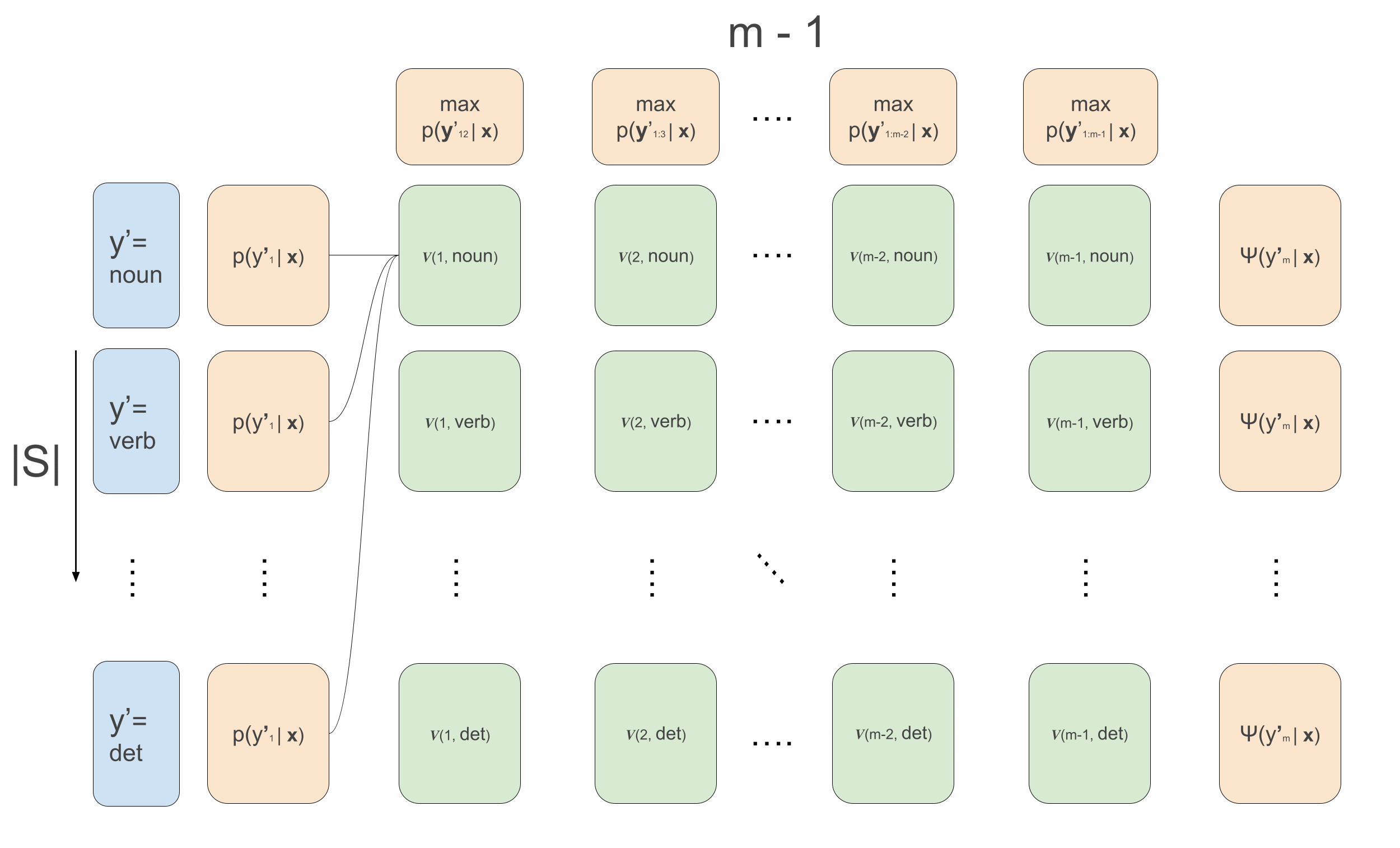
\[\begin{aligned} \alpha(1, y^{\prime}_2) &= \sum_{y^{\prime}_1}\psi(y^{\prime}_1, \mathbf{x}, 1) \cdot \psi(y^{\prime}_1, y^{\prime}_{2}) \\ \alpha(t, y^{\prime}_{t+1}) &\leftarrow \sum_{y^{\prime}_{t}}\psi(y^{\prime}_t, \mathbf{x}, t) \cdot \psi(y^{\prime}_t, y^{\prime}_{t+1})\cdot \alpha(t-1, y^{\prime}_t) \end{aligned}\]

For Viterbi we do exactly the same thing but replace the sums by max, and we need to keep track of which of the previous \(y\)’s maximized the current recursion. We will call these values ‘backpointers’, because in the backward pass we’ll use them to trace back the maximizing sequence.

\[\begin{aligned} v(1, y^{\prime}_2) &= \max_{y^{\prime}_1}\psi(y^{\prime}_1, \mathbf{x}, 1) \cdot \psi(y^{\prime}_1, y^{\prime}_{2}) \\ v(t, y^{\prime}_{t+1}) &\leftarrow \max_{y^{\prime}_{t}}\psi(y^{\prime}_t, \mathbf{x}, t) \cdot \psi(y^{\prime}_t, y^{\prime}_{t+1})\cdot v(t-1, y^{\prime}_t) \\ \overleftarrow{v}(1, y^{\prime}_2) &= arg\max_{y^{\prime}_1}\psi(y^{\prime}_1, \mathbf{x}, 1) \cdot \psi(y^{\prime}_1, y^{\prime}_{2}) \\ \overleftarrow{v}(t, y^{\prime}_{t+1}) &\leftarrow arg\max_{y^{\prime}_{t}}\psi(y^{\prime}_t, \mathbf{x}, t) \cdot \psi(y^{\prime}_t, y^{\prime}_{t+1})\cdot v(t-1, y^{\prime}_t) \\ \end{aligned}\]

Note that again here, we are using the conditional independence relations for efficient decoding. If there were no conditional independence relations, we would unfortunately need to calculate the likelihood of all possible sequences, but here we use it to our advantage and recursively maximize. In the below animation we can see the computations done in the forward- and backward-pass of Viterbi. We initialize the leftmost green boxes by taking the maximum of the initial values \(\max_{y^{\prime}_1}\bar{p}(y^{\prime}_1 \mid \mathbf{x}) = \max_{y^{\prime}_1}\psi(y^{\prime}_1, \mathbf{x}, 1) \cdot \psi(y^{\prime}_1, y^{\prime}_{2})\). At the final column we can start actually decoding and decide what the maximizing final POS tag is: \(\hat{y}^{\prime}_m = arg\max_{y^{\prime}_m}\psi(y^{\prime}_m) \cdot v_{m-1}(y^{\prime}_m)\). This also gives us the backpointer to follow to get the best path backwards, giving the maximizing sequence: \(\hat{y}^{\prime}_t \leftarrow \overleftarrow{v}_t(\hat{y}^{\prime}_{t+1})\) \(\forall t \in \{m-1, 1\}\).

Putting it all together

Yay, that’s all the ingredients!

We discussed that for some applications it’s useful to model the dependencies among the output variables, which asks for structured prediction. In this case we chose a linear-chain conditional random field, which is simply a probabilistic graphical model with a particular choice of parametrized feature-functions as factors. We showed how to learn the parameters of the model by maximizing the likelihood. This procedure asked for an efficient way of calculating the partition function and the marginals of the CRF model, which we did with the dynamic programming algorithm belief propagation. Finally we showed how to find the maximizing sequence under the current model with the Viterbi algorithm. Now we are ready to implement everything in PyTorch, and use a deep neural network as a feature extractor. We can simply put the CRF on top of a neural network of choice, like LSTM’s, and train everything end-to-end with stochastic gradient ascent on the likelihood! All part of part two and part three of this series.

Sources

The following sources I heavily used for this post:

The original CRF paper
John D. Lafferty, Andrew McCallum, and Fernando C. N. Pereira. Conditional random fields: Probabilistic models for segmenting and labeling sequence data. In Proceedings of the Eighteenth International Conference on Machine Learning, ICML ’01, pages 282–289, San Francisco, CA,USA, 2001. Morgan Kaufmann Publishers Inc.

The absolutely awesome introduction to CRFs by Charles Sutton and Andrew McCallum.
Charles Sutton and Andrew McCallum. An introduction to conditional random fields. Found.Trends Mach. Learn., 4(4):267–373, April 2012.

Hugo Larochelle’s tutorial on YouTube. Clearest explanation to be found about CRFs afaik!