Learning in High Dimension Always Amounts to Extrapolation

In this post I’ll attempt to shed some light on the conclusion that is drawn (in part¹) from the above image:

We shouldn’t use interpolation/extrapolation in the way the terms are defined below when talking about generalization, because for high dimensional data deep learning models always have to extrapolate, regardless of the dimension of the underlying data manifold.

The image is taken from Balestriero, Pesenti, and LeCun, 2021 and the goal of this post is to reproduce it. In the process of doing that, we hopefully get a better understanding of what the interpolation/extrapolation debate (here and here and here) is about. To be honest, the whole debate is not going to be any clearer after reading this post. David Hume describes quite nicely what is probably going on in this discussion in his “an enquiry concerning human understanding”:

It might reasonably be expected, in questions, which have been canvassed and disputed with great eagerness, since the first origin of science and philosophy, that the meaning of all terms, at least, should have been agreed upon among the disputants; and our enquiries, in the course of two thousand years, have been able to pass from words to the true and real subject of the controversy. For how easy may it seem to give exact definitions of the terms employed in reasoning, and make these definitions, not the mere sounds of words, the object of future scrutiny and examination? But if we consider the matter more narrowly, we shall be apt to draw a quite opposite conclusion. From this circumstance alone, that a controversy has been long kept on foot, and remains still undecided, we may presume, that there is some ambiguity in the expression, and that the disputants affix different ideas to the terms employed in the controversy.

Basically, it seems like a lot of arguments between people are a result of not properly defining what is discussed (and the last author on this paper probably agrees). I never read Hume, but adding a fancy philosopher quote is a necessary step towards creating the illusion that I know what I’m talking about. In reality, the reason I’m writing this blogpost is because I didn’t understand the Learning in High Dimension paper at all on first reading. With this post I hope to get a better understanding of it, and share that understanding.

At the end this post, we will hopefully know more about the following terms:

• The curse of dimensionality
• Convex hull
• Ambient dimension
• Intrinsic dimension / data manifold dimension
• Interpolation / extrapolation

The Key Idea

The key idea in this paper is that we shouldn’t be using interpolation and extrapolation (in the way the terms are defined in this paper) as indicators of generalization performance, because models are likely extrapolating. That is true even for data manifolds with moderate intrinsic dimensions. What counts is the dimensionality of the data representation, which is often much higher than the intrinsic dimension. The authors think researchers that equate generalization with extrapolation should develop appropriate geometrical definitions of extrapolation that actually align with generalization in the context of high dimensional data. So let’s dive in!

When are we interpolating?

In this section: Interpolation, Extrapolation, Convex Hull, Convex Combination, Linear Combination, Curse of Dimensionality

The definition of interpolation in the paper is the following:

Definition 1. Interpolation occurs for a sample \(\mathbf{x}\) whenever this sample belongs to the convex hull of a set of samples \(\mathbf{X} \triangleq \{\mathbf{x}_1, \dots, \mathbf{x}_N\}\), if not, extrapolation occurs.

So what is the convex hull of a set of samples?

A vector \(\mathbf{x}\) lies within the convex hull of a set of samples \(\mathbf{x}_1, \dots, \mathbf{x}_N\) if we can write it as a convex combination of the samples:

\[\mathbf{x} = \lambda_1 \mathbf{x}_1 + \dots + \lambda_N \mathbf{x}_N\]

Subject to the constraints: \(\lambda_i \geq 0\) and \(\sum_i \lambda_i = 1\). Let’s have a look at what that means in a dimension we can still visualize.

# Make up some samples that happen to form a nice square in R2.
hull_samples = np.array([[1, 1],
                         [2, 1],
                         [2, 2],
                         [1, 2]])
                         
# Here's a point that is a convex combination of the hull samples ..
point_in_hull = np.array([[1.5, 1.5]])

# .. and here's one that isn't.
point_outside_hull = np.array([[2.5, 2]])

# Calculate the convex hull with scipy.spatial.ConvexHull.
hull = ConvexHull(hull_samples)

# Let's plot it.
plt.plot(hull_samples[:, 0], hull_samples[:, 1], 'o', c='navy')
plt.plot(point_in_hull[:, 0], point_in_hull[:, 1], 'o', c='lightgreen')
plt.plot(point_outside_hull[:, 0], point_outside_hull[:, 1], 'o', c='tomato')
for simplex in hull.simplices:
  plt.plot(hull_samples[simplex, 0], hull_samples[simplex, 1], 'k')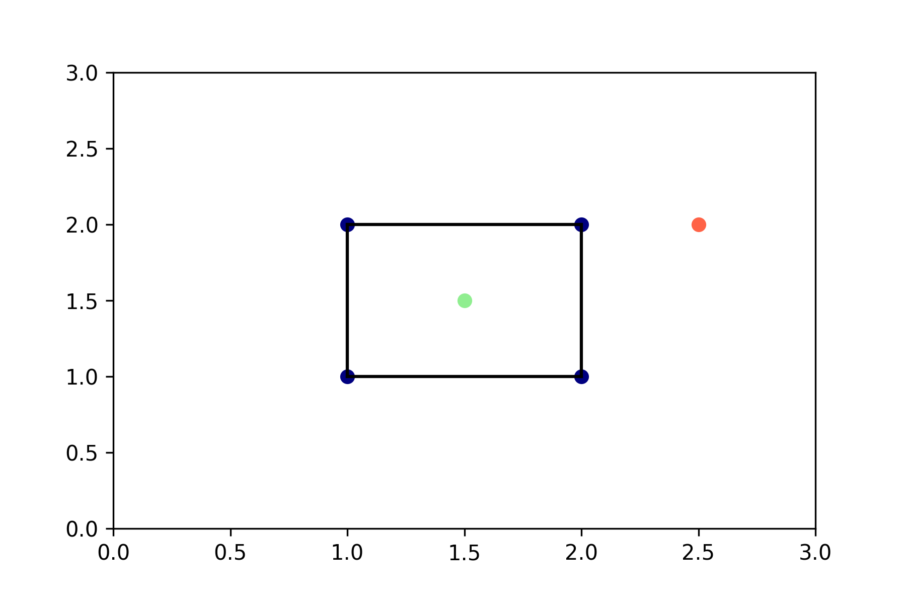

Everything within (or on) this square is a convex combination of the convex hull of the four samples, everything outside it but still in \(\mathbb{R}^2\) is a linear combination of the samples, relaxing the constraints on the \(\lambda_i\)’s. Note that we can easily calculate the probability of lying within the convex hull of samples here if we assume that all values will lie between zero and three. Let’s say we sample points uniformly between zero and three for both dimensions, then the probability that a new sample lies within the convex hull of the four ‘training’ samples is the area of the convex hull divided by the total area:

\[p(\mathbf{x} \in \text{Hull}(\mathbf{X})) = \frac{1}{9}\]

In general, for a convex hull with area \(c\) in \(\mathbb{R}^2\) and data points in \([x_0, x_1]\) the probability of lying in the convex hull of the four training samples is \(\frac{c}{(x_1 - x_0)^2}\).

Now let’s see what happens if we move to three dimensions. We’ll stretch out the square from above into a cube and calculate the probability of lying within this cube.

fig = plt.figure()
ax = plt.axes(projection='3d')

# Make the cube of 3D hull points (8 points, each is a corner of the cube).
X = np.array([1, 2, 2, 1, 1, 2, 2, 1])
Y = np.array([1, 1, 2, 2, 1, 1, 2, 2])
Z = np.array([1, 1, 1, 1, 2, 2, 2, 2])

# Set the same limits as the 2D example.
ax.set_xlim(0, 3)
ax.set_ylim(0, 3)
ax.set_zlim(0, 3)

# A function to get a convex combination of a set of points.
def convex_combination(points):
  lambdas = np.random.randint(0, 10, len(points))
  lambdas_n = lambdas / np.sum(lambdas)
  return np.dot(points.transpose([1, 0]), lambdas_n)

# A function to get an linear combination of a set of points 
# that is *not* a convex combination.
def linear_combination(points):
  lambdas = np.random.randint(0, 10, len(points))
  lambdas_n = lambdas / np.sum(lambdas)
  offset = np.random.choice([np.random.uniform(-0.1, -0.02),
                             np.random.uniform(0.02, 0.1)])
  lambdas_n = lambdas_n + offset
  return np.dot(points.transpose([1, 0]), lambdas_n)

# Plot some convex combinations of the hull data points.
for i in range(10):
  num_points = np.random.randint(5, 8, 1)
  point_indices = np.random.randint(0, 8, num_points)
  points = np.array([X[point_indices], 
                     Y[point_indices], 
                     Z[point_indices]]).transpose([1, 0])
  new_point = convex_combination(points)
  ax.scatter(*new_point, c='lightgreen', zorder=2.5)

# Plot some linear combinations of the hull data points.
for i in range(10):
  num_points = np.random.randint(5, 8, 1)
  point_indices = np.random.randint(0, 8, num_points)
  points = np.array([X[point_indices], 
                     Y[point_indices], 
                     Z[point_indices]]).transpose([1, 0])
  new_point = linear_combination(points)
  ax.scatter(*new_point, c='tomato', zorder=12.5)

# Plot the box around the convex hull.
ax.plot(X, Y, Z, 'o', c='navy', zorder=7.5)
for i in range(4):
  idx = i
  idx_right = (idx + 1) % 4
  ax.plot([X[idx], X[idx_right]],
          [Y[idx], Y[idx_right]],
          [Z[idx], Z[idx_right]], color = 'k', zorder=10)
  ax.plot([X[idx+4], X[idx_right+4]],
          [Y[idx+4], Y[idx_right+4]],
          [Z[idx+4], Z[idx_right+4]], color = 'k', zorder=10)
  ax.plot([X[idx], X[idx_right+3]],
          [Y[idx], Y[idx_right+3]],
          [Z[idx], Z[idx_right+3]], color = 'k', zorder=10)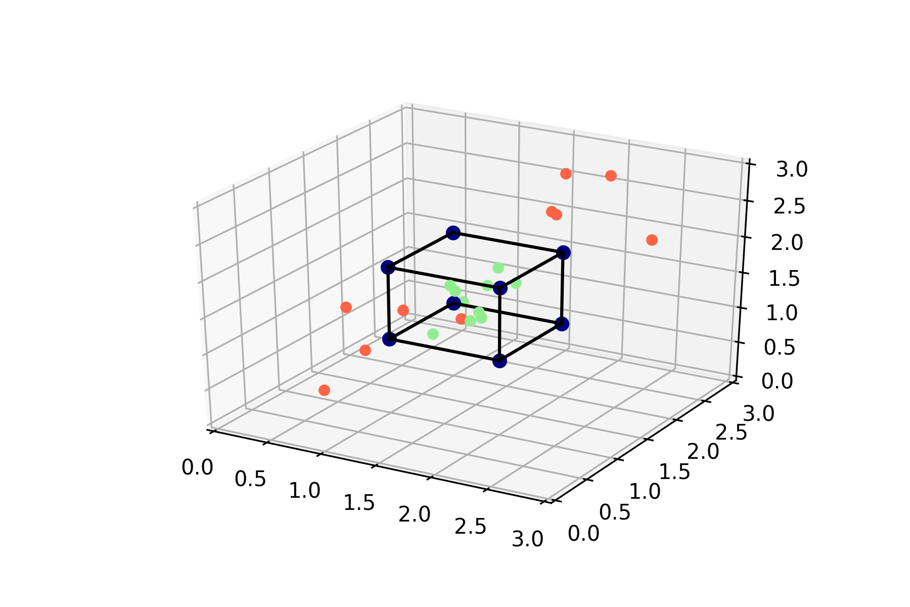

This cube has a volume of one, and the probability of lying within this cube has become:

\[p(\mathbf{x} \in \text{Hull}(\mathbf{X})) = \frac{1}{27}\]

In general, for a convex hull with volume \(c\) in \(\mathbb{R}^3\) and data points in \([x_0, x_1]\) the probability of lying in the convex hull is \(\frac{c}{(x_1 - x_0)^3}\). This provides some intuition as to why the probability of lying within the convex hull (i.e., being in interpolation regime) quickly goes down as the dimensionality of the problem goes up – exponentially quickly.

This intuition is formalized in the paper by a theorem describing the limiting behaviour of the probability of lying in the convex hull for new (i.i.d.) samples from a Gaussian.

Theorem 1 (Baranay and Furedi, 1988). Given a \(d\)-dimensional dataset \(\mathbf{X} \triangleq \{\mathbf{x}_1, \dots, \mathbf{x}_N\}\) with i.i.d. samples \(\mathbf{x}_n \sim \mathcal{N}(0, \mathbb{I}_d)\), for all \(n\), the probability that a new sample \(\mathbf{x} \sim \mathcal{N}(0, \mathbb{I}_d)\) is in interpolation regime (recall Def. 1) has the following limiting behavior:

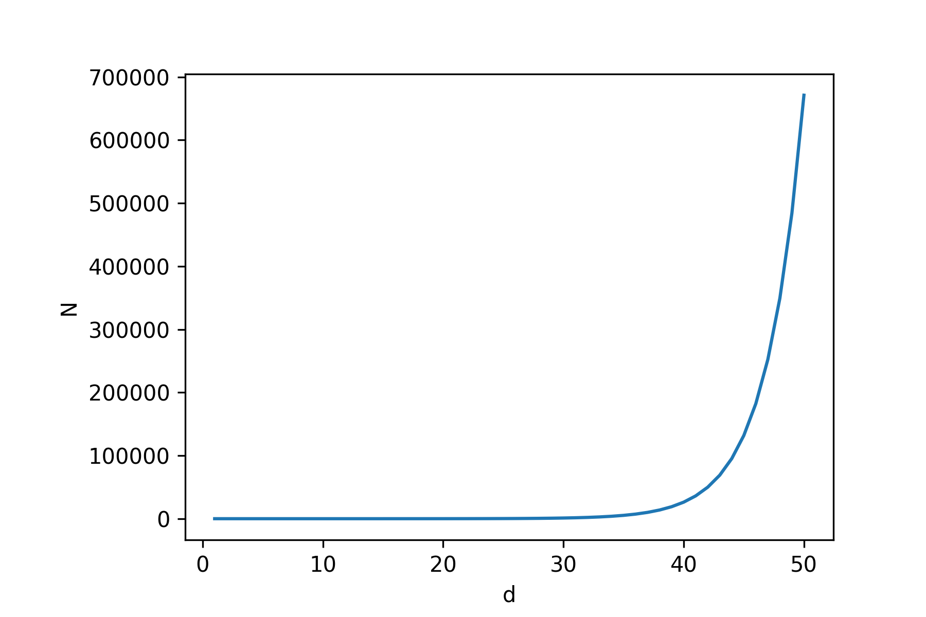
\[\lim_{d \rightarrow \infty} p(\mathbf{x} \in \text{Hull}(\mathbf{X})) = \begin{cases} 1 & \text{if } N > d^{-1}2^{d/2} \\ 0 & \text{if } N < d^{-1}2^{d/2} \end{cases}\]

This theorem says that the probability that a new sample lies in the convex hull of \(N\) samples
tends to one for increasing dimensions if \(N > d^{-1}2^{d/2}\), but if \(N\) is smaller, it tends to 0. This means we need to exponentially increase the number of datapoints \(N\) for increasing \(d\) if we want to have a chance at being in interpolation regime. See below for a plot of the minimal \(N\) needed per dimension \(d\) (\(N = d^{-1}2^{d/2}\)).

In this section we learned what the convex hull of datapoints is, and what it means to be interpolating or extrapolating w.r.t. the convex hull of samples. We got some intuition about the curse of dimensionality, and might already see why it is pretty unlikely for a new sample to be in interpolation regime of real-world datasets. We are ready to start reproducing the first plot.

Going further, we should keep in mind that the following sentences are equivalent:

• The new sample lies in the convex hull of training samples.
• The new sample is within interpolation regime of the training samples.
• The new sample is a convex combination of training samples.

Reproducing the First Plot

In this section: Ambient Dimension

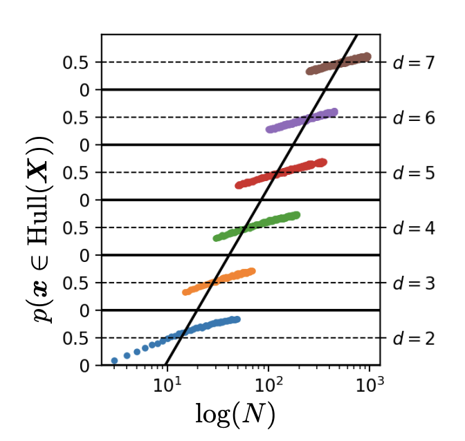
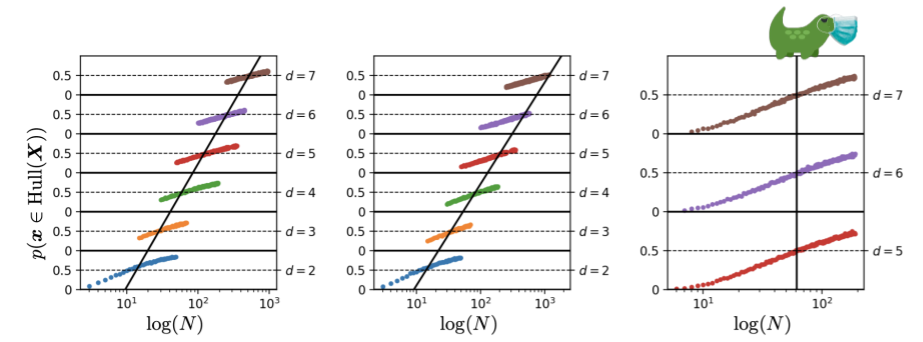
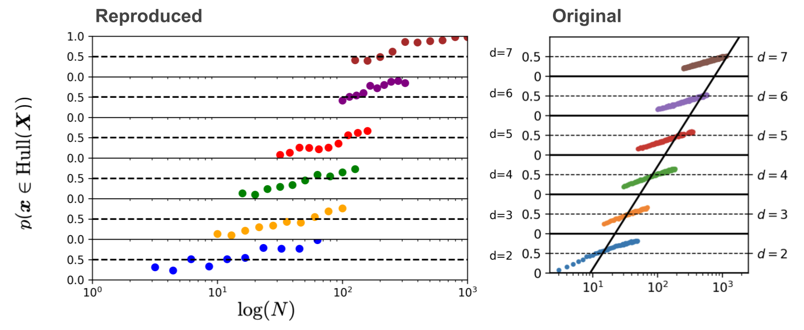
This image is a stack of six plots. Each plot shows the estimated probability that a new sample from a Gaussian with dimension \(d\) will lie in the convex hull of \(N\) training samples of this Gaussian. For example, for the bottom plot the estimated probability that a new sample \(\mathbf{x} \sim \mathcal{N}(0, \mathbb{I}_2)\) lies in the convex hull of the \(N = 10\) samples \(\mathbf{x}_1, \dots, \mathbf{x}_{10} \sim \mathcal{N}(0, \mathbb{I}_2)\) is roughly 50%. For a gaussian with dimensionality 7 we already need more than \(10^{2.4} \approx 250\) training examples to have roughly 50% chance of a new sample being in the convex hull of those training examples. The black line through the six plots is the line that denotes how \(N\) should change to keep the probability of a new sample being in the convex hull of 50% for increasing dimension \(d\). This shows that the necessary number of datapoints \(N\) increases exponentially with \(d\), because it’s a straight line through a logarithmic scale.

This dimension \(d\) of the Gaussian is called the ambient dimension. The ambient dimension of the data is the number of dimensions we use to represent it. If we take the well-known MNIST dataset as an example, the ambient dimension that is often used is the number of pixels: \(d = 28 \times 28 = 784\).

How to get the estimate of being in the convex hull?
We want to reproduce the above image, so how do we estimate the probability of being in the convex hull for a new sample? The authors of the paper use a Monte-Carlo estimate. For each of the six plots above, we can do the following to get a single point on the line. Sample \(N\) points from a Gaussian with dimension \(d\) to form a training set of samples: \(\mathbf{x}_1, \dots, \mathbf{x}_{N}\). Then, sample a new point \(\mathbf{x} \sim \mathcal{N}(0, \mathbb{I}_d)\) and determine whether it lies in the convex hull of the training set. Repeat this whole thing 500,000 times, giving 500,000 binary decisions whether the sample was inside the hull or not. The average of this gives the Monte-Carlo estimate of the probability that a new sample lies in the convex hull of the training set – a single point on the plot. To get the entire plot we need to do this for \(N\) between 1 and \(10^3 = 1000\) for every \(d\). You can imagine that this will take a while, so we will cheat the estimate slightly and only sample the convex hull once for every of the 500,000 trials we do per value for \(N\). Additionally, we only take \(10\) different values for \(N\) for each \(d\).

Below, we’ll implement everything to do this. We are going to need a few functions:

• sample_from_gaussian: a function to sample from a multivariate Gaussian.
• is_in_convex_hull_batch: returns vector of boolean values that specify whether each sample in a batch of new vectors fall inside the convex hull.
• probability_in_convex_hull_batch: returns the estimated probability that a new sample lies in the convex hull of training samples.

def sample_from_gaussian(num_samples: int, num_dimensions: int, mu=0,
                         sigma=1) -> np.array:
  """
  Sample num_samples from a multivariate Gaussian with `num_dimensions`
  independent dimensions.

  Returns: [num_samples, num_dimensions] gaussian samples.
  """
  mu, sigma = np.zeros(num_dimensions) + mu, np.identity(num_dimensions) * sigma
  return np.random.multivariate_normal(mu, sigma, num_samples)

samples = sample_from_gaussian(1000, 3)

# Plot the 3 independent dimensions of the samples.
plt.hist(samples[:, 0], bins=25, density=True, alpha=0.5, color='g')
plt.hist(samples[:, 1], bins=25, density=True, alpha=0.5, color='b')
plt.hist(samples[:, 2], bins=25, density=True, alpha=0.5, color='r')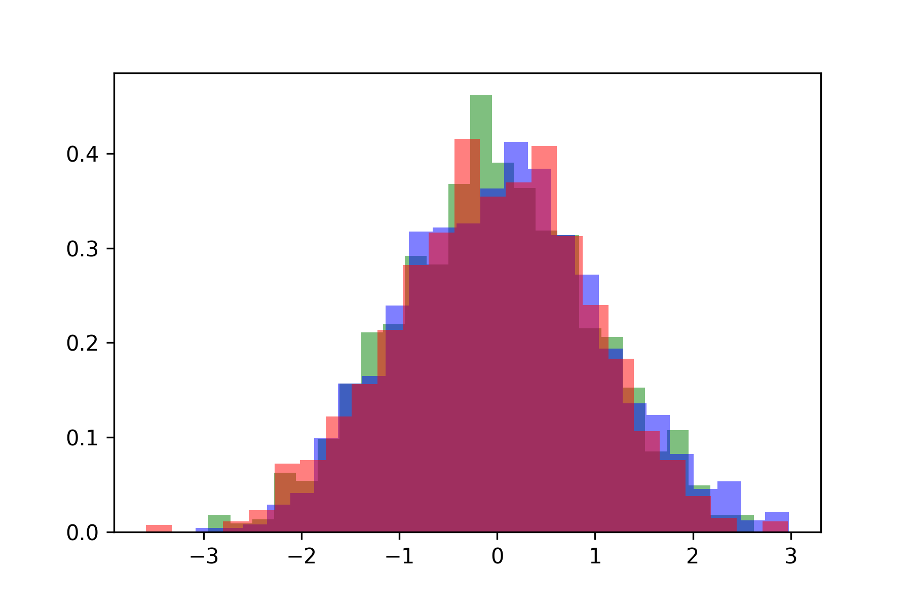

Above you see a three overlapping histograms plotted, one for each of the dimensions of the sampled Gaussians.

Probability of lying in the convex hull
Recall that a vector \(\mathbf{x}\) lies within the convex hull spanned by samples \(\mathbf{x}_1, \dots, \mathbf{x}_N \in \mathbb{R}^d\) if we can write it as a convex combination of the samples \(\mathbf{x} = \lambda_1\mathbf{x}_1 + \dots + \lambda_N\mathbf{x}_N\) subject to \(\lambda_i \geq 0\) and \(\sum_i \lambda_i = 1\).

Now to find out whether a new point \(\mathbf{x}\) is in the convex hull we just need to verify whether it is a convex combination of the hull samples. This can be framed as a quadratic programming problem, and that’s what we will do for the second plot below, but for the first plot we can use a very simple batched implementation using SciPy.

The QP problem is necessary for the second plot since the method used below does not work for degenerate convex hull spaces, which will be the case for the second plot (lower intrinsic dimension than ambient dimension). Don’t worry if these terms don’t mean anything to you yet, I’ll explain them later.

Below we use a batched implementation of finding whether points lie in the convex hull by relying on scipy.Delaunay.

def is_in_convex_hull_batch(new_samples: np.array, 
                            hull_samples: np.array) -> np.array:
  """
  Returns a vector of size new_samples.shape[0] (the number of new samples),
  with a boolean indicating whether or not the sample lies in the convex hull.
  """
  assert new_samples.shape[1] == hull_samples.shape[1],  \
  "Dimensions of new sample and convex hull samples should be the same, "
  "but are %d and %d" % (new_samples.shape[1], samples.shape[1])
  if not isinstance(hull_samples, Delaunay):
    hull = Delaunay(hull_samples)
  return hull.find_simplex(new_samples) >= 0

def probability_in_convex_hull_batch(new_samples: np.array, 
                                     hull_samples: np.array) -> float:
  """
  The first dimension is the number of new samples, the second dimension
  is the dimensionality of the vector.
  """
  in_convex_hull = is_in_convex_hull_batch(new_samples, hull_samples)
  return np.sum(in_convex_hull) / new_samples.shape[0]

Let’s see if it works for the convex hull we visualized above in \(\mathbb{R}^2\). In addition to the point inside and the point outside the hull above, let’s add two more points outside the hull to get a quarter of the points inside the hull.

point_in_hull = np.array([1.3, 1.8])
point_outside_hull = np.array([3, 2])
point_outside_hull_2 = np.array([4, 2])
point_outside_hull_3 = np.array([0, 2])
points = np.concatenate([np.expand_dims(point_in_hull, axis=0),
                         np.expand_dims(point_outside_hull, axis=0),
                         np.expand_dims(point_outside_hull_2, axis=0),
                         np.expand_dims(point_outside_hull_3, axis=0)], axis=0)
print("Probability inside hull (batch method): ", 
      probability_in_convex_hull_batch(points, hull_samples))

>> Probability inside hull (batch method): 0.25

Now we are ready to reproduce the first plot. We sample \(N\) points for an ambient dimension \(d\) from a multivariate Gaussian \(\mathcal{N}(\mathbf{0}, \mathbb{I}_d)\). These points form the convex hull. Then we sample 500,000 new points (num_trials) from the same Gaussian, and see whether they fall within the hull, or outside, to estimate the probability of being inside the convex hull.

We do this for different \(N\) per dimensions \(d \in \{2, \dots, 7\}\). The N below (in num_convex_hull_samples_per_dim) are chosen to roughly be the same as in the plot (I eyeballed it).

NB: note that the code below runs reasonably quick for dimensions 2 to 6, but takes a few minutes for dimensions = 7.

# The different ambient dimensions that we will consider.
ambient_dimensions = list(range(2, 8))

# The different values for N that we will consider.
num_dataset_sizes = 10
num_convex_hull_samples_per_dim = [np.logspace(0.5, 1.8, num_dataset_sizes),
                                   np.logspace(1, 2, num_dataset_sizes),
                                   np.logspace(1.2, 2.1, num_dataset_sizes),
                                   np.logspace(1.5, 2.2, num_dataset_sizes),
                                   np.logspace(2, 2.5, num_dataset_sizes),
                                   np.logspace(2.1, 3, num_dataset_sizes)]
num_trials = 500000

def get_convex_hull_probability_gaussian(num_trials: int, dataset_size: int, 
                                         ambient_dimension: int) -> float:
  """Samples `dataset_size` samples from a Gaussian of dimension 
  `ambient_dimension`, and then calculates for `num_trials` new samples
  whether they lie on the convex hull or not. Returns the estimated
  probability that a new sample lies in the convex hull."""
  convex_hull_samples =  sample_from_gaussian(num_samples=dataset_size, 
                                              num_dimensions=ambient_dimension)
  new_samples = sample_from_gaussian(num_samples=num_trials, 
                                     num_dimensions=ambient_dimension)
  p_new_samples_in_hull = probability_in_convex_hull_batch(
      new_samples=new_samples, hull_samples=convex_hull_samples)
  return p_new_samples_in_hull

# For each ambient dimension d, get the probability that a new sample lies in
# the convex hull per value for N.
all_probabilities = np.zeros([len(ambient_dimensions),
                              num_dataset_sizes])
for dimension_idx, dimension in enumerate(ambient_dimensions):
  print("Working on %d-D" % dimension)
  num_convex_hull_samples = num_convex_hull_samples_per_dim[dimension_idx]
  for size_idx, dataset_size in enumerate(num_convex_hull_samples):
    probability_in_hull = get_convex_hull_probability_gaussian(
        num_trials, int(dataset_size), dimension)
    all_probabilities[dimension_idx, size_idx] = probability_in_hull

>> Working on 2-D
>> Working on 3-D
>> Working on 4-D
>> Working on 5-D
>> Working on 6-D
>> Working on 7-D

Open to see the function plot_probabilities() to plot this (very uninteresting).

def plot_probabilities(x_space_per_dimension, dimensions, probabilities):
  """
  x_space_per_dimension: [len(dimensions)] an np.logspace per dimension
  dimensions: the different dimensions to be plotted on the Y-axis
  probabilities: [num_dimensions, num_dataset_sizes] convex hull probabilities
  """
  num_dimensions = len(dimensions)
  fig = plt.figure()

  # All stacked plots equally high.
  gridspecs = gridspec.GridSpec(num_dimensions, 1, 
                                height_ratios=[1] * num_dimensions) 

  # Loop over the grids and plot the probabilities for a dimension in each.
  colors = ["b", "orange", "g", "r", "purple", "brown"]
  for i, ax in enumerate(reversed(list(gridspecs))):
    x = x_space_per_dimension[i]
    ax = plt.subplot(ax)
    ax.set_xscale("log")
    ax.set_xlim(1, 10**3)  # Hardcode the limits for each subplots here.
    ax.scatter(x, probabilities[i], color=colors[i])
    ax.set_ylim(0, 1)

    # Only add the Y tick for p=1 at the topmost subplot.
    if i < (dimensions[-1] - dimensions[0]):
      ax.set_yticks([0, 0.5], minor=False)
    else:
      ax.set_yticks([0, 0.5, 1], minor=False)
    
    # Only add the X ticks for the bottom subplot.
    if i != 0:
      ax.set_xticks([])
    else:
      ax.set_xlabel('log(N)', fontsize = 12)
      ax.xaxis.set_label_coords(0.5, -0.655)

    # Some annotations.
    plt.axhline(y=0.5, color='black', linestyle='--')
    plt.text(10**3+500,0.5,'d=%d' % dimensions[i] ,rotation=0)

  # Remove vertical gap between subplots.
  plt.ylabel("p(x in Hull)", fontsize=12)
  plt.subplots_adjust(hspace=.0)
  plt.show()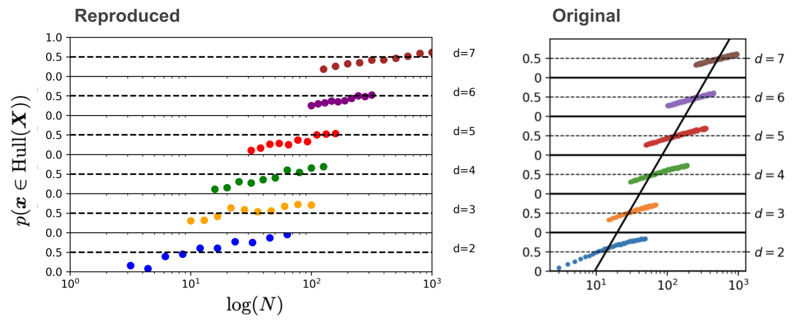

Jippie²! There it is! So beautiful. Very reproduce. Much similar.

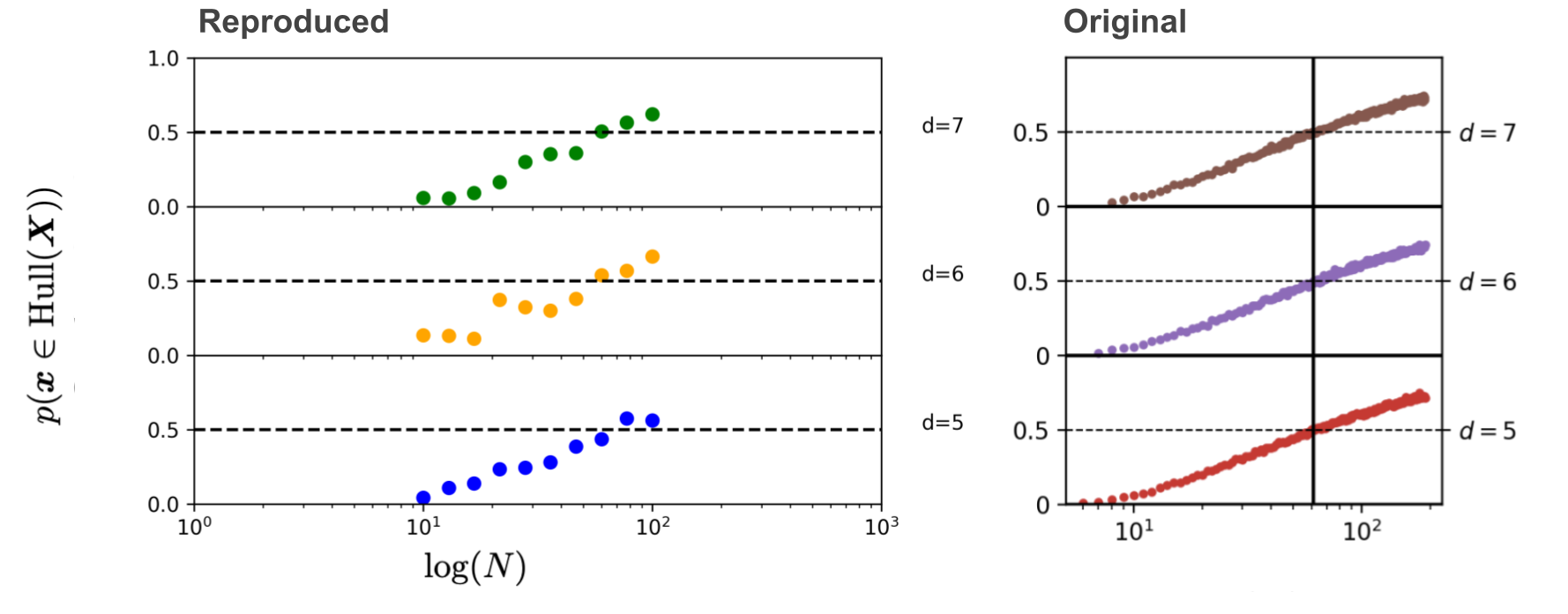
Reproducing the Second Plot

In this section: Intrinsic Dimension, Data Manifold, Quadratic Programming

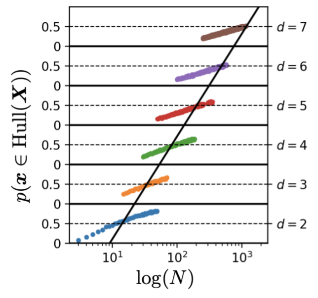
This plot looks incredibly similar to the first one. The difference lies in the underlying data manifold that is sampled from, i.e. the intrinsic dimension (denoted by \(\bar{d}\)) will be different. For the first plot, we sampled from a \(d\)-dimensional Gaussian. The intrinsic dimension of this Gaussian was the same as the dimension we used to represent it: \(d = \bar{d}\). For this plot, we sample 1-dimensional data and represent it in a higher dimension (\(d \in \{2, \ldots, 7\}\)). In each case the representation takes the form of a nonlinear differentiable manifold (\(\bar{d} = 1\)). The point of the plot is to show that even for data with a 1-dimensional manifold, if the ambient dimension goes up, you will still need exponentially more data to stay in interpolation regime with a high probability.

So how are we going to sample from a nonlinear differentiable 1-dimensional data manifold with a higher dimension \(d\)? We’ll take the following steps.

• Sample \(d\) independent Gaussian points.
• Interpolate between these points with a spline to get a 1D data manifold.
• Sample from a uniform distribution between 0 and 1 and put these through the spline to get samples.

These samples are now taken from a spline \(f: \mathbb{R} \rightarrow \mathbb{R}^{d}\), meaning the ambient dimension will be \(d\), whereas the intrinsic dimension is 1.

Why would this work?

This works because \(d\) independent samples will almost surely span all of \(\mathbb{R}^d\), so that the dimension of the samples and, hence, the resulting spline is \(d\).

def construct_one_dimensional_manifold(ambient_dimension: int):
  """
  ambient_dimension: what dimension should the data be represented in

  Returns: The spline function f: R -> R^ambient_dimension.
  """
  # We take dimensions+2 for the dimension of the Gaussian because otherwise 
  # the scipy interp1d function doesn't work.
  gaussian_points = sample_from_gaussian(num_samples=ambient_dimension, 
                                         num_dimensions=ambient_dimension+2)
  x = np.linspace(0, 1, num=ambient_dimension+2, endpoint=True)
  f = interp1d(x, gaussian_points, kind='cubic')
  return f

def sample_from_one_dimensional_manifold(manifold_func, num_samples):
  return manifold_func(np.random.uniform(low=0, high=1, size=num_samples))

Now we can sample from 1-dimensional manifolds in any ambient dimension. We can’t visualize dimensions above 3, but we can look at the first two components of the spline. Below let’s sample from the manifold in 2 and 10 dimensions.

spline_2d = construct_one_dimensional_manifold(ambient_dimension=2)
spline_10d = construct_one_dimensional_manifold(ambient_dimension=10)

# Plot some samples from this manifold for d=2 and d=10.
x = np.linspace(0, 1, num=10, endpoint=True)
plt.plot(spline_2d(x)[0, :], spline_2d(x)[1, :])
plt.plot(spline_10d(x)[0, :], spline_10d(x)[1, :])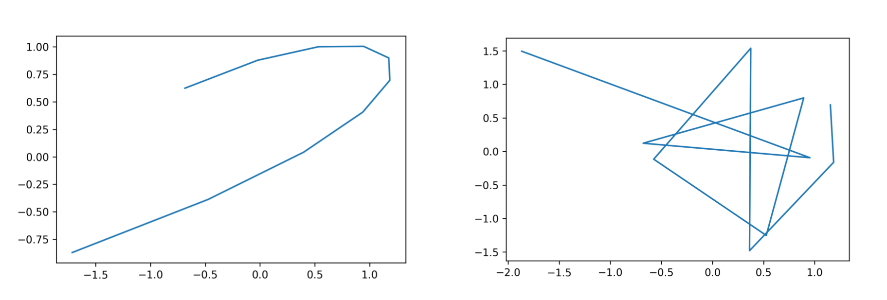

In the above image one can see that the spline represented in 10 dimensions on the right is much more wobbly than the one that has ambient dimension 2; both have intrinsic dimension 1.

Does it lie in the convex hull? A QP problem

Unfortunately, the batched method for finding out whether a new point lies inside the convex hull doesn’t work anymore. This is because our samples all come from a 1D manifold, which causes geometric degeneracy. From the SciPy docs:

QhullError 
Raised when Qhull encounters an error condition, such as geometrical degeneracy 
when options to resolve are not enabled.

Instead, we will frame it as a quadratic programming problem³ and solve it with a QP solver that can handle degeneracy.

We want to find the coefficients such that \(\boldsymbol{\lambda}_1 \mathbf{x}_1 + \dots + \boldsymbol{\lambda}_N \mathbf{x}_N = \mathbf{x}\). The constraints on the \(\boldsymbol{\lambda}\)’s also need to be taken care of. If we can find coefficients that satisfy these constraints, the new point \(\mathbf{x}\) lies in the convex hull.

Recall what we have already defined so far:

• \(N\) the number of convex hull samples
• \(d\) the ambient dimension
• \(\boldsymbol{\lambda} \in \mathbb{R}^{N}\) the convex combination coefficients
• the convex hull samples \(\mathbf{X} \in \mathbb{R}^{N \times d}\)
• the new sample \(\mathbf{x} \in \mathbb{R}^d\)

Our quadratic program problem is the following:

\[\begin{align} \text{min}_{\boldsymbol{\lambda}} &\left(\mathbf{X}^T\boldsymbol{\lambda} - \mathbf{x}\right)^T \left(\mathbf{X}^T\boldsymbol{\lambda} - \mathbf{x}\right) \\ s.t. & \sum_i \lambda_i = 1 \\ & \lambda_i \geq 0 \end{align}\]

If we solve this QP problem, and \(\left(\mathbf{X}^T\boldsymbol{\lambda} - \mathbf{x}\right)^T \left(\mathbf{X}^T\boldsymbol{\lambda} - \mathbf{x}\right) = 0\), it means we have \(\mathbf{x} = \mathbf{X}^T\boldsymbol{\lambda}\), and our new sample is a convex combination of the samples, i.e. lies in the convex hull.

We can rewrite the objective to the standard form as follows:

\[\begin{align} \text{min}_{\boldsymbol{\lambda}} &\frac{1}{2}\boldsymbol{\lambda}^T(\mathbf{X}\mathbf{X}^T)\boldsymbol{\lambda} + (-\mathbf{X}\mathbf{y})^T\boldsymbol{\lambda} \end{align}\]

This follows from the fact that multiplying by a constant doesn’t change the objective, and neither does a constant addition. For the QP library that we are going to use, we need to rewrite the inequality constraints into the form \(G\boldsymbol{\lambda} \leq h\). To this end we define the matrix \(G\) as follows:

\[G = \begin{pmatrix} -1 & 0 & 0 & 0 \\ 0 & -1 & 0 & 0\\ 0 & 0 & -1 & 0\\ 0 & 0 & 0 & -1 \end{pmatrix}\]

and the vector \(h\):

\[h = \begin{pmatrix} 0\\ 0\\ 0\\ 0 \end{pmatrix}\]

The equality constraint needs to be written into the form \(A\lambda = b\):

\[A = \begin{pmatrix} 1 & 1 & 1 & 1 \\ \end{pmatrix}\]

and the vector \(b\):

\[b = \begin{pmatrix} 1 \end{pmatrix}\]

This ensures that the sum of the \(\lambda_i\) equals 1 and all entries are non-negative.

Below we implement this, and we assume a new vector is in the complex hull if the QP problem has a ‘loss’ smaller than 1e-5 (meaning \(\left(\mathbf{X}^T\boldsymbol{\lambda} - \mathbf{x}\right)^T \left(\mathbf{X}^T\boldsymbol{\lambda} - \mathbf{x}\right) \leq 1e-5\)).

Note the definitions of the following variables in the code below to keep it the same as in the example that I used.

\[\mathbf{P} := \mathbf{X}\mathbf{X}^T\] \[\mathbf{q} := -\mathbf{X}\mathbf{y}\]

# You can ignore this function; it's a wrapper around the QP solver.
def cvxopt_solve_qp(P, q, G=None, h=None, A=None, b=None):
  "Copied from https://scaron.info/blog/quadratic-programming-in-python.html"
  P = .5 * (P + P.T)  # make sure P is symmetric
  args = [cvxopt.matrix(P), cvxopt.matrix(q)]
  if G is not None:
      args.extend([cvxopt.matrix(G), cvxopt.matrix(h)])
      if A is not None:
          args.extend([cvxopt.matrix(A), cvxopt.matrix(b)])
  sol = cvxopt.solvers.qp(*args)
  if 'optimal' not in sol['status']:  # Failed
      return np.array([-10] * P.shape[1]).reshape((P.shape[1],))
  return np.array(sol['x']).reshape((P.shape[1],))
  
def is_in_convex_hull_qp(new_sample: np.array, hull_samples: np.array) -> bool:
  """
  :param new_sample: [num_dimensions]
  :param hull_samples: [num_hull_samples, num_dimensions]

  Calcs for `new_sample` whether it lies in the convex hull of `hull_samples`.
  """
  num_hull_samples = len(hull_samples)
  num_dimensions = len(new_sample)

  # Define the QP problem.
  P = np.dot(hull_samples, hull_samples.T).astype(np.double)
  q = -np.dot(hull_samples, new_sample).astype(np.double)

  G = -np.identity(num_hull_samples)
  h = np.array([0] * num_hull_samples).astype(np.double)

  A = np.ones([1, num_hull_samples]).astype(np.double)
  b = np.array([1]).astype(np.double)

  result = cvxopt_solve_qp(P, q, G, h, A, b)

  def loss(l_i, sign=1., y=new_sample, X=hull_samples):
    return sign * np.dot((y - np.dot(X.T, l_i)).T, (y - np.dot(X.T, l_i)))

  l = loss(result)
  if l < 1e-5:
    return True
  else:
    return False

def probability_in_convex_hull_qp(new_samples: np.array, 
                                  hull_samples: np.array) -> float:
  """
  The first dimension is the number of new samples, the second dimension
  is the dimensionality of the sample. Returns the estimated probability
  that a new sample lies in the convex hull of `hull_samples`.
  """
  in_convex_hull = np.zeros([new_samples.shape[0]])
  for i in range(len(new_samples)):
    new_sample = new_samples[i, :]
    vec_in_convex_hull = is_in_convex_hull_qp(new_sample, hull_samples)
    in_convex_hull[i] = vec_in_convex_hull
  return np.sum(in_convex_hull) / new_samples.shape[0]

Let’s test it again for the example points and convex hull that we also used above (probability should be \(\frac{1}{4}\)).

print("Probability inside hull (quadratic programming method): ", 
      probability_in_convex_hull_qp(points, hull_samples))

>> Probability inside hull (quadratic programming method): 0.25

We’re ready to reproduce the figure. We take the following steps to do so:

1. Sample a spline for a dimension \(d \in \{2, \ldots, 7\}\).
2. Get \(N\) convex hull samples from this same spline.
3. Get a new sample from the spline.
4. See whether it’s in the convex hull of the \(N\) samples by solving the quadratic programming problem.
5. Repeat num_trials times.

CAVEAT: The code below is incredibly slow, because of the new method of finding whether a point is in the convex hull used; framing it as a QP problem. The paper does 500,000 trials, but below we do just 100, to be a bit faster (runs in a few minutes). It still works, but obviously the estimate is much worse.

ambient_dimensions = list(range(2, 8))
num_dataset_sizes = 10
num_convex_hull_samples_per_d = [np.logspace(0.5, 1.8, num_dataset_sizes),
                                 np.logspace(1, 2, num_dataset_sizes),
                                 np.logspace(1.2, 2.1, num_dataset_sizes),
                                 np.logspace(1.5, 2.2, num_dataset_sizes),
                                 np.logspace(2, 2.5, num_dataset_sizes),
                                 np.logspace(2.1, 3, num_dataset_sizes)]

num_trials = 100

def get_convex_hull_probability(manifold_spline, num_trials: int, 
                                dataset_size: int, 
                                ambient_dimension: int) -> float:
  # Get the samples to form the convex hull.
  hull_samples = manifold_spline(np.random.uniform(low=0, high=1,
                                                   size=dataset_size))

  # Get new samples from the manifold.                          
  new_samples = manifold_spline(np.random.uniform(low=0, high=1,
                                                  size=num_trials))

  # Estimate the probability that a new sample lies in the convex hull.
  p_new_samples_in_hull = probability_in_convex_hull_qp(
      new_samples=new_samples.transpose(),
      hull_samples=hull_samples.transpose())
  return p_new_samples_in_hull

# Loop over all ambient dimensions.
all_probabilities_2 = np.zeros([len(ambient_dimensions),
                                num_dataset_sizes])
for dimension_idx, dimension in enumerate(ambient_dimensions):
  print("Working on %d-D" % dimension)
  dataset_sizes = num_convex_hull_samples_per_d[dimension_idx]

  # Sample a new spline for this ambient dimension.
  spline = construct_one_dimensional_manifold(ambient_dimension=dimension)

  # Loop over the different dataset sizes.
  for size_idx, dataset_size in enumerate(dataset_sizes):

    # Estimate the probability.
    probability_in_hull = get_convex_hull_probability(spline, num_trials,
                                                      int(dataset_size),
                                                      dimension)
    all_probabilities_2[dimension_idx, size_idx] = probability_in_hull

>> Working on 2-D
>> Working on 3-D
>> Working on 4-D
>> Working on 5-D
>> Working on 6-D
>> Working on 7-D

We can see that even though we cheated by only sampling the data points once per ambient dimension, and only doing 100 Monte-Carlo trials instead of 500,000, we get away with it!

Reproducing the Final Plot

In this section: Convex Hull Dimension

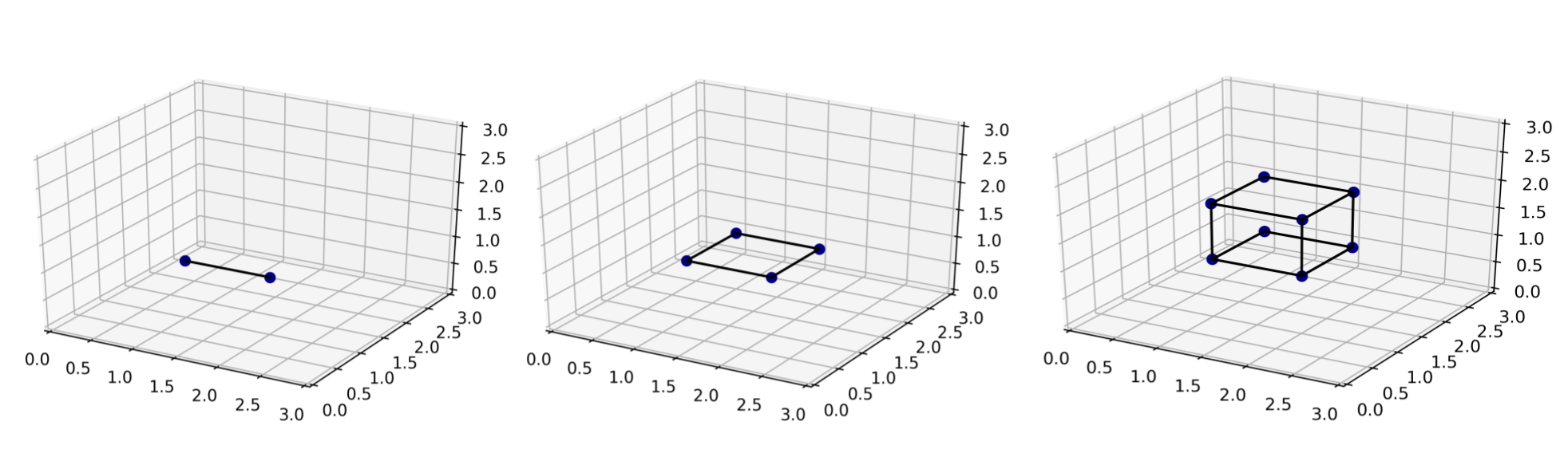
The final plot requires the introduction of some new terminology; it’s the plot that answers the question: “so how can we control the probability of interpolating, i.e. of a new sample lying in the convex hull”? The answer is (somewhat unsurprisingly now); by keeping the dimensions of the convex hull fixed. The convex hull dimension, also referred to as the dimension of the lowest dimensional affine subspace including the entire data manifold in the paper, is the dimension of the convex hull of the data points. Recall the discussion of what the convex hull is above? Below on the left we take two of those datapoints, that happen to lie on a line in \(\mathbb{R}^3\), so the ambient dimension is 3, but the convex hull dimension is 1; it’s a line. If we take 4 points that lie on a plane, like in the middle below, we have ambient dimension of 3 and convex hull dimension of 2. Finally, if we take the full set of 8 data points, we get a convex hull dimension of 3, which equals the ambient dimension. This convex hull dimension is denoted by \(d^*\) in the paper.

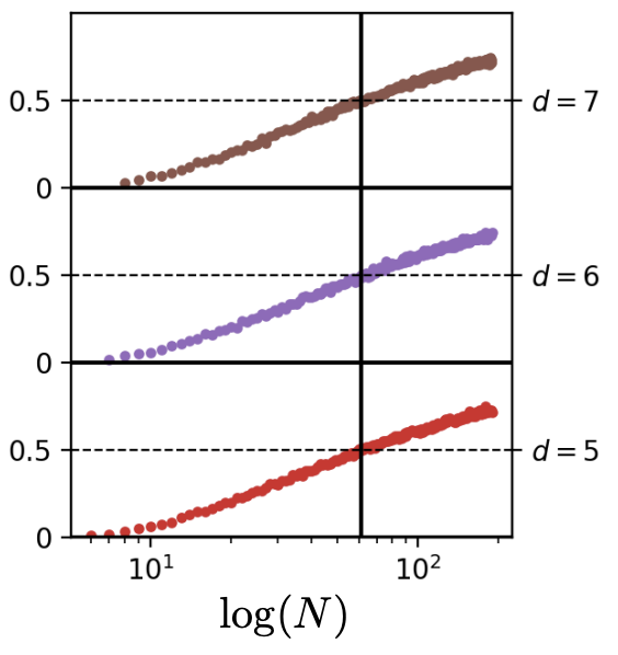
Now what we do to reproduce the final plot, is show that if we keep the convex hull dimension \(d^*\) similar, but increase the ambient dimension, it doesn’t have the effect it had before anymore! We don’t need more datapoints \(N\) to keep the probability of a new sample lying in the convex hull at 50% for a higher ambient dimension. The paper uses a convex hull dimension of \(d^* = 4\) and ambient dimensions of \(d \in \{5, 6, 7\}\)

How to control the convex hull dimension, while increasing the ambient dimension?

We’ll use the same intuition about Gaussians as before. To get 4-dimensional data we sample 4 independent Gaussian data points, these points will very likely have a convex hull dimension of 4. To see why, imagine the 3D plots from above. If we sample two data points in this 3D space, we can get at most a convex hull dimension of 1 (a line), then if we sample another point and it happens to be an extension of this line, the convex hull dimension won’t increase, it’ll still be a line. The chances of this happening are zero, so the dimension will increase to 2, a plane. Then if you sample another point, it will again not be an extension of the plane. If we generalize this intuition to higher dimensions, we obtain that the probability of sampling a new point from a Gaussian that lies on the convex hull is zero (whenever the dimension of the convex hull is small than the dimension of the ambient space).

To increase the ambient dimension without increasing the convex hull dimension, we can simply multiply the data points of a lower dimension with an invertible matrix of the desired dimension. This way we won’t increase the convex hull dimension (since \(rank(AB) = \min(rank(A), rank(B))\)), but we will increase the ambient dimension. We’re basically just embedding a 4D gaussian into a higher dimensional space.

For example, we have \(N\) samples from the 4D Gaussian \(\mathbf{X} \in \mathbb{R}^{N \times 4}\) (with \(rank(\mathbf{X}) = 4\)), and we want to embed these in an ambient dimension of \(d=7\). We add 3 columns of zeros to \(\mathbf{X}\) to get \(\hat{\mathbf{X}} \in \mathbb{R}^{N \times 7}\) (still with \(rank(\hat{\mathbf{X}}) = 4\)), multiply it with the sampled invertible matrix \(\mathbf{A} \in \mathbb{R}^{7 \times 7}\), giving us the final samples \(\mathbf{X}^{\star} \in \mathbb{R}^{N \times 7}\) (with \(rank(\mathbf{X}^{\star}) = rank(\hat{\mathbf{X}}\mathbf{A}) = \min(rank(\hat{\mathbf{X}}), rank(\mathbf{A})) = 4\)).

To get a random invertible matrix of \(d\times d\) we just sample \(d\) times from a \(d\)-dimensional Gaussian again, which guarantees to give an invertible matrix (with the same intuition as above). Let’s implement it!

def is_invertible(matrix: np.array):
  assert matrix.shape[0] == matrix.shape[1], "Non-square matrix cannot be " \
  "invertible."
  if np.linalg.cond(matrix) < 1 / sys.float_info.epsilon:
    return True
  else:
    return False

def get_invertible_matrix(num_dimensions: int):
  matrix = sample_from_gaussian(num_dimensions, num_dimensions)
  if is_invertible(matrix):
    return matrix
  else:
    raise ValueError("Sampled non-invertible matrix.")

def make_d_dimensions(samples: np.array, invertible_matrix: np.array,
                      new_dimensions: int) -> np.array:
  """
  samples: [num_samples, num_dimensions]
  invertible_matrix: [new_dimensions, new_dimensions]
  new_dimensions: the number of output dimensions

  Uses an invertible matrix to project input samples into a higher dimensional
  space.
  
  Returns: 
    [num_samples, new_dimensions] the new samples in a higher dimension
    [new_dimensions, new_dimensions] the transformation matrix used
  """
  assert len(samples.shape) == 2, "Need 2D matrix for argument 'samples'."
  assert new_dimensions > samples.shape[1], \
  "Cannot increase to %d dimensions if existing dimensions is %d" % (
      new_dimensions, samples.shape[1])
  existing_dimensions = samples.shape[1]
  extra_dimensions = new_dimensions - existing_dimensions
  
  # We add columns of zeros to the samples to be able to multiply
  # them with the right dimension invertible matrix.
  add_zeros = np.zeros([samples.shape[0], extra_dimensions])
  concat_samples = np.concatenate([samples, add_zeros], axis=1)
  
  # Transform the samples into a higher-dimensional space.
  new_samples = np.dot(concat_samples, invertible_matrix)
  
  # Check that we can recover the old samples.
  old_samples_recovered = np.dot(new_samples, np.linalg.inv(invertible_matrix))
  assert np.allclose(old_samples_recovered, concat_samples)
  
  return new_samples

def sample_4d_gaussian(num_samples: int, invertible_matrix: np.array,
                       ambient_dimension: int):
  """Samples data with a convex hull dimension of 4 and an ambient dimension
  of `ambient_dimension`."""
  gaussian_samples = sample_from_gaussian(num_samples=num_samples, 
                                          num_dimensions=4)
  return make_d_dimensions(gaussian_samples, invertible_matrix, 
                           new_dimensions=ambient_dimension)

Now we’re finally ready to reproduce the final figure.

ambient_dimensions = list(range(5, 8))
num_dataset_sizes = 10
num_convex_hull_samples_per_d = [np.logspace(1, 2, num_dataset_sizes),
                                 np.logspace(1, 2, num_dataset_sizes),
                                 np.logspace(1, 2, num_dataset_sizes)]

num_trials = 1000

def get_convex_hull_probability(num_trials: int, dataset_size: int, 
                                ambient_dimension: int) -> float:
  # Sample the invertible matrix for this ambient dimension.
  matrix = get_invertible_matrix(ambient_dimension)
  
  # Get the convex hull samples of.
  hull_samples = sample_4d_gaussian(num_samples=dataset_size, 
                                    invertible_matrix=matrix,
                                    ambient_dimension=ambient_dimension)
  
  # Get the new samples.
  new_samples = sample_4d_gaussian(num_samples=num_trials, 
                                   invertible_matrix=matrix,
                                   ambient_dimension=ambient_dimension)
  
  # Estimate the probability of lying in the convex hull.
  p_new_samples_in_hull = probability_in_convex_hull_qp(
      new_samples=new_samples,
      hull_samples=hull_samples)
  return p_new_samples_in_hull

all_probabilities_3 = np.zeros([len(ambient_dimensions),
                                num_dataset_sizes])
for dimension_idx, dimension in enumerate(ambient_dimensions):
  print("Working on %d-D" % dimension)
  dataset_sizes = num_convex_hull_samples_per_d[dimension_idx]
  for size_idx, dataset_size in enumerate(dataset_sizes):
    probability_in_hull = get_convex_hull_probability(num_trials,
                                                      int(dataset_size),
                                                      dimension)
    all_probabilities_3[dimension_idx, size_idx] = probability_in_hull

>> Working on 5-D
>> Working on 6-D
>> Working on 7-D

And we’re done! If it’s also a thorn in your eye that the colors of these plots don’t match, go check out the code for this blogpost for yourself and change it!

Final Ponderings

What we learned now that no matter what the intrinsic dimension of your underlying data manifold is, for increasing convex hull dimensions we need exponentially more data to have any chance of being in interpolation regime. Now at this point, that doesn’t sound too surprising anymore, since we defined interpolation regime as the convex hull. But that’s precisely what this paper has achieved, it illuminated some of the terms that were previously undefined in the debate, and made them unsurprising. Of course you might say that everything is very different for real-world data and for expressive deep learning models that have a much better behaved representation space for this data. What the authors show however in the paper beyond the figure we reproduced here, is that the same conclusions hold. Despite the likely lower dimensional intrinsic data manifold of natural images, finding samples in interpolation regime becomes exponentially difficult with respect to the considered ambient data dimension. Current deep learning methods almost surely operate in an extrapolation regime in both the data and their embedding space. Now of course, like the authors of this paper also acknowledge, this doesn’t mean that deep learning methods are perfect. What definition for interpolation/extrapolation should we then take if we are talking about generalization performance? Perhaps here there’s one answer from another researcher. I would be interested to see more. If you have comments or questions, don’t hesitate to reach out on my twitter.

Acknowledgements

If you want to be a computer scientist like me and still be able to understand concepts from mathematics, take the following steps:

1. Meet a cute boy at a houseparty
2. Find out he’s doing a PhD in maths
3. Motivate said cute boy / maths PhD to become your boyfriend
4. Quarantine together during a global pandemic
5. Pester him with questions about convex hulls
6. ???
7. Profit

Additionally, I’m grateful for comments from Randall Balestriero, Robert Kirk, and Aryaman Fasciati.

Sources

Randall Balestriero and Jerome Pesenti and Yann LeCun (2021). Learning in High Dimension Always Amounts to Extrapolation

Barany, I. and Furedi, Z. (1988). On the shape of the convex hull of random points.

1. The experiments that mostly endorse this conclusion are the experiments on real datasets in the paper. ↩

2. Jippie means “Yippie” in Dutch. ↩

3. You could also frame it as a linear programming problem. ↩